Basic Analyses
Additional Information on Quantile Regression
Quantile regression models the relationship between a specified conditional quantile (or percentile) of a dependent (response) variable and one or more independent (explanatory) variables (Cade and Noon 2003). For example, modeling the 50th quantile of a response variable produces the median line under which 50% of the observed responses are located, and modeling the 90th quantile produces a line under which 90% of the observed responses are located below (in Figure 1).
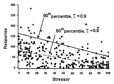 Figure 1. Quantile regression of matched data for a stressor and a response with the 50th and 90th percentiles noted.
Like conventional linear regression, a common functional form that is assumed for a quantile regression analysis may be a linear model:
![]() where yτ denotes the τth quantile of y, βi are constant coefficients, x1 is the explanatory variable. Quantile regressions can have more than one explanatory variable, but we limit the following discussion to the univariate case.
where yτ denotes the τth quantile of y, βi are constant coefficients, x1 is the explanatory variable. Quantile regressions can have more than one explanatory variable, but we limit the following discussion to the univariate case.
Quantile regression as illustrated in Figure 1 is a semi-parametric method (i.e., combines parametric and nonparametric methods). A given quantile may be assumed related linearly to the independent (response, Y-axis) variable, but the distribution of Y at a given X is not assumed to have a normal distribution. Moreover, other specific assumptions, such as homogeneity of variance do not apply.
Quantile regression is robust to outliers in dependent (response, Y-axis) variables, but is sensitive to points sparsely distributed toward the extremes of the independent (explanatory, X-axis) variables. In cases where such leverage points are present, one may do a weighted quantile regression. The influence of outliers, censored data, data clusters, and leverage points may be evaluated by comparing plots after removing (or, in the case of leverage points, weighting) these points. Any data pruning of this nature must be transparently described. In general, the points should remain on the plot with flags indicating whether they were weighted or omitted from the model.
Is the Assumed Functional Form Appropriate?
Although non-linear quantile regression analyses are available, a simplifying assumption is that the relationships being modeled are linear with respect to the explanatory variables. In Figure 1, the relationships between response variable and the explanatory variable is assumed to be linear. In many cases, a linear relationship is a reasonably accurate estimate of the actual relationship, if there is no reason to believe differently. Most biotic metrics are generally considered to change linearly in relation to stressor gradients, but ecological knowledge of the underlying processes may help one select alternate functional forms.
Are there Other Assumptions with Quantile Regression?
An assumption for using the 90th percentile is that the data wedge often observed in scatter plots of biological metrics is the result of other stressors co-occurring with the modeled stressor which cause additional decline in biological response over the stressor gradient.
If data from the impaired site are located far outside the upper boundary determined from regional data, it may be an indication that the comparison to the regional data is not valid. This situation can arise for a variety reasons. For example, field sampling methods applied at the impaired site may differ significantly from those applied to collect the regional data. In general, large outliers should be inspected carefully to determine whether they can be usefully compared to regional data.