Basic Principles & Issues
Additional Information on Interpreting Statistics
Statistical Significance
In general, a statistical test has the following components. (1) A null hypothesis is formulated. This is usually a probability model that assumes no effect of interest, any apparent effects being attributable to chance. (2) A test statistic is chosen, which will be computed from results of the experiment to quantify how strongly the results contradict the null hypothesis. (3) Once the study has been conducted, the p-value is the probability of any result that contradicts the null hypothesis as strongly as the results actually obtained, based on the value of the test statistic.
Statistical tests and their associated p-values are easily misunderstood. Analysts who are not confident of their grasp of statistical tests will benefit from review of a transparent example, such as the "lady tasting tea" (Fisher 1956).
| Lady Tasting Tea | ||||||||||||||||||
|---|---|---|---|---|---|---|---|---|---|---|---|---|---|---|---|---|---|---|
|
For this example, the null hypothesis is that the lady is guessing which cups had tea or milk added first. Our test statistic will be the number of cups correctly identified as "tea first". The p-value, then, is the probability of a test statistic (correctly labeled cups of tea) being as large as the value of the test statistic actually obtained, if the the null hypothesis is true. The results of the experiment should be evaluated using criteria associated with low chance of false positives, in this case, lucky guesses. Let us say that all cups have been labeled correctly. What is the chance of doing this well by random guessing? There are 8! / 4!(8-1)! = 70 possible ways of labeling the cups, but only one that is completely correct. Therefore, the probability of correctly labeling all cups at random is 1/70, or 0.014. The value 0.014 is our p-value (according to convention, we may write p = 0.014). The null hypothesis is rejected according to the usual criterion p ≤ 0.05. Now suppose that the taster labeled some cups correctly and others incorrectly. We may wonder if the outcome suggests some deviation from random guessing. We display below the probabilities, according to the random-guessing model, of labeling a given number of cups "tea first."
Suppose, for example, that three cups labeled "tea first" did in fact have tea added to the cup first, while one of them had milk added first. (By implication, three cups labeled "milk first" also had milk added to the cup first). The p-value in this case is probability of getting that outcome, or any other outcome that provides as strong evidence for a deviation from random guessing. To our previous value of 0.014 (the probability of all correct guesses) we add the probability 0.229 (the probability of one incorrect label of each type). Therefore, we report p = 0.24. In this case, the taster has not established an ability to do better than random guessing, according to the customary criterion for statistical significance. Note that due to the small number of trials, the test has low power: In order to obtain a statistically significant result, the taster must evaluate every cup correctly. |
||||||||||||||||||

The p-value from a test is not the probability of truth or untruth of a hypothesis. It is the probability of data that contradict the null hypothesis as strongly as the data actually obtained, if the null hypothesis is true.
It should be noted that, in Fisher's example of the lady tasting tea, the investigator adopts a skeptical attitude towards the claim of discrimination ability and places a burden of proof on the claim. This is typical of research settings, where the researcher hopes to show that an effect has been observed that cannot be attributed to variation in the data. In general, care should be taken that the use of statistical test results are not associated with an inappropriate burden of proof. If one can identify a magnitude of effect that can be treated as biologically important, such as a critical percentage change of a variable relative to reference conditions, the assistance of a statistician may be sought in performing a procedure determining whether or not the 'biologically important' effect can be rejected, in lieu of the standard test of a no-effect null hypothesis.
Confidence intervals, discussed below, can be used to analyze data without assumptions about the relative burden of proof for different outcomes.
| Testing for effect size of practical significance |
|---|
| Special types of statistical tests may be more useful in a regulatory situation, if there is a policy of considering a specific effect magnitude to have regulatory (i.e., practical) significance, say a 10% change in the mean value of a biological response. Instead of testing a null hypothesis of zero effect, one may test that the effect is no smaller a 10% change in mean, placing a burden of proof on the position that effects are unimportant. CADDIS methodology, on the other hand, is largely directed towards determination of whether particular stressors can account for observed ecological impairment. |
Statistical Tests and Randomized Experiments
Although causal assessments may be based largely on observational data, some consideration of perspectives during planning of a randomized experiment may be helpful in understanding statistical testing concepts. At the planning stage, a test statistic is tentatively identified that will be computed from results of the experiment and used in deciding what outcome to report for the experiment. In our example, the number of cups that the subject will classify correctly is used to accept or reject the subject's claim. A cutoff (critical) value of the test statistic is identified, such that the chance of some erroneous conclusions is acceptably low.
Indeed, the experimenter hopes for a low chance of finding an effect, if there really is no effect, i.e., a low chance of a false positive. According to the null hypothesis, the treatments may be viewed simply as random labeling of experimental units. If the experimenter has decided to enforce a 5% chance of a false positive, use of the critical p-value of 0.05 is justified as just a matter of checking that results satisfy a pre-specified criterion, before claiming to have observed something of interest. In addition, the experimenter hopes that if there are substantial effects of the treatment, there will be a substantial probability of finding statistical significance, i.e., that the test will have good power.
| When the test is not significant: more on the role of statistical power |
|---|
|
By itself, a large p-value simply indicates inconclusive results, brought about by some combination of a small effect and high variability or a low quantity of data. As noted earlier a large p-value does not provide evidence that the null hypothesis is supported by the data. Some analysts emphasize supplementing a statistical test with an evaluation of statistical power. One particular power approach is the minimal detectable difference (MDD). The MDD is the size of actual effect associated with a given test power. The power of a test depends on the magnitude of deviation from the null hypothesis. Designing a test with adequate sensitivity generally involves deciding on a parameter that represents the magnitude of effect, for example the relative difference between the mean of a response variable, in treated versus control groups. (In the lady-tasting-team scenario, an effect size can be formulated in terms of odds of correct and incorrect labels.) The chance of statistically significant results should increase with the size of the effect. While the value of power calculations appears undisputed in the context of planning studies, some authors discourage the use of power calculations as an approach to data analysis, usually suggesting that a more straightforward interpretation can be based on a confidence interval for the size of effect. |
Confidence Intervals
A 95% confidence interval has the following interpretations: (1) There is a 95% chance of the true value of the parameter falling within the interval; (2) Values outside the interval can be rejected on the basis of a two-sided statistical test with alpha 5%.
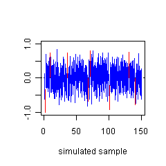 Figure A1. The proper interpretation of a confidence interval can be illustrated based on a Monte Carlo simulation. See text for details.The first interpretation means, technically, that a confidence interval computed from a random sample has a 95% of including the true parameter value. This can be illustrated using Monte Carlo simulation, as in the following example (see Sokal and Rohlf 1981). We generated random data by drawing a sample of size 25 from a normal population with mean zero and variance one, and computing the standard normal-theory confidence interval for the mean from the simulated data. Figure A1 displays confidence intervals based on 150 independent repetitions. For each simulated data set, we determined whether the confidence interval did or did not enclose the true mean (which is zero, indicated with a horizontal dotted line). In Figure 2, the blue bars correspond to confidence intervals that enclose the true mean, the red bars to intervals that do not. When we repeated the random sampling, the confidence interval included the true mean for 958 of 1000 random samples, close to the true 95% coverage for the procedure.
Confidence intervals are likely to be more easily interpreted than statistical tests in some situations. A large p-value, by itself, is ambiguous, as previously noted. A confidence interval may be more informative, displaying an estimated effect along with a measure of statistical uncertainty (which will be large in case of few or variable data). Unlike statistical tests, confidence intervals are neutral regarding the relative "burden of proof" to be associated with various hypotheses about effect sizes.
Graphical display of confidence intervals is particularly encouraged in comparative contexts, such as when comparing results among successive years of monitoring. p-values are likely to be more difficult to compare.
Applying confidence intervals in a stressor-response context may require that the analyst specify a magnitude of effect that would ecologically meaningful. For example, one might specify a priori that a decrease in total richness of 5 taxa would constitute an ecologically meaningful decrease. Then, one would examine the estimated mean effect of a stressor on total taxon richness and its associated confidence intervals to ascertain whether this threshold was exceeded.
General Recommendations for the Use of Statistical Tests and Confidence Intervals
- Methods that assume normality should not be applied to data that contain outliers or have heavy-tailed distributions. Rank-based or other outlier-resistant methods may be applied, without needing to exclude putative outliers from the analysis.
- Methods that assume normality may be applied to data with skew distributions if the data are transformed to correct skewness.
- Assessment of distributional assumptions should be based in part on graphical evaluation of distributions and familiarity and experience with particular types of variables, and not only on statistical tests of assumptions. It is often of interest to know in what way a distribution deviates from normality, e.g., because of outliers or skewness. The normal distribution should not be treated as a default in cases where experience indicates that, say, a particular type of variable is more likely to have a lognormal distribution.
- Possible effects of and remedies for autocorrelation or pseudoreplication should be considered.
- When focusing on effects of one variable, possible effects of other variables should be taken into account. It is desirable to consider methods that minimize confounding. Some standard methods for evaluating the effects of a single variable on a response, while ignoring others may not be suitable for ecological data.
- In a regression context, tests of assumptions are generally applied to regression residuals (differences between observed values of the Y variable, and values predicted by the model).
- Correct use of statistical tests and confidence intervals requires that the appropriate interpretation be kept in mind. In particular, statistical significance (a low p-value) is conceptually distinct from practical significance, i.e., from the issue of whether biological effects observed in a situation are large enough in magnitude to be of practical importance.
More Information
- The paper "mathematics of a lady tasting tea" (Fisher 2000; first published 1956) is currently available online. The story is included in a similarly-titled, engaging book by Salsburg (2001), useful for understanding many aspects of statistical data analysis.
- Relatively advanced, rigorous treatments of statistical testing include Cox and Hinkley (1974) and Cox (2006). For understanding of the role of randomization (or probabilistic sampling), it is helpful to explore the concept of design- versus model-based analysis (Cox 2006, Ch. 9; Little 2004). In essence, certain statistical inferences may be considered "robust" because of a justification based on the known randomization scheme, rather than by a basis in distributional assumptions.
- Miller (1997) is useful with respect to practical consequences of violating assumptions of statistical tests, in particular reduction in power associated with outliers or heavy-tailed distributions.
- Hoenig and Heisey (2001) criticize the use of power computations in data analysis, while acknowledging that they are necessary in study design (also see Cox and Hinkley 1974, p. 105).
- Some readers will note that the account given here is frequentist, and may think that more attention could be given to alternatives to conventional statistical tests (of null hypotheses of zero effect), such as Bayesian methods, likelihood ratios, meta-analysis, confidence intervals, or non-standard statistical tests. Here, the priority is avoiding unjustified interpretations of data based on misunderstandings of standard methods. The treatment is not intended to discourage alternative approaches.
- An important trend in ecological statistics, is model comparisons using likelihood and information-theoretical methods. It is valuable to be able to approach causal issues based on comparisons of fitted models. For example, testing that effects of land-use can be accounted for by stressors that result from land-use changes might be formulated as a comparison of models that are similar except with respect to the inclusion of a land-use variable. Model comparisons are used based on likelihood-ratio tests (including partial F tests as a special case) or on use of penalized likelihood statistics such as the Akaike Information Criterion (AIC). Burham and Anderson (2002) is an influential text. Bolker (2008) is a resource for ecological model comparisons in the programming language R.
- Graphical display of confidence intervals is encouraged over p-values, which are likely to be more difficult to compare.
- Stunkard (1994) provides a treatment of tests for which the null hypothesis is a specified magnitude of effect, rather than the conventional zero-effect null hypothesis.