Nutrient and Response Variable Overviews

Descriptions of common nutrient (e.g., nitrogen) and response variables (e.g., phytoplankton) and sampling methods for these variables. Click on a variable below for more information. Additional resources for variables and sampling methods are included.

• Clarity

  Clarity is a measure of the amount of sunlight that can penetrate through the water column, reflecting the amount of dissolved colored or suspended material in any waterbody. Clarity can be affected by natural and introduced materials. Clarity can be the result of, as well as a limitation to, productivity. Suspended algae contribute to reduced water clarity, which at the same time can limit light available to growth of algae at depth. In streams and lakes, inorganic sediment can also contribute to reduced clarity. Although usually the case following storms, some waters do maintain high inorganic sediment loads even during baseflow. In the context of nutrient criteria, the utility of clarity measures is related to contributions from suspended algal material in the water column. This material can come from true phytoplankton or from tychoplankton (algae dislodged or sloughed from the benthos). In either case, significant correlations have been drawn between the amount of algae in the water column and its clarity, especially for lakes. One of the common trophic indices for lakes, the Trophic State Index (TSI), can be derived using a measure of transparency. Clarity may have limitations as a nutrient endpoint as reduced clarity is often caused by non-nutrient issues such as waste discharges, runoff from watersheds, soil erosion, and humic acids and other organic compounds resulting from the decay of plants and leaf litter.

  Clarity can be measured in a number of ways. One of the traditional lake quality measures is the vertical Secchi depth transparency measurement, which was adapted from a method developed by an Italian papal advisor, Father Pietro Angelo Secchi, in the 19th century. Similar horizontal adaptations of transparency measures have been tested for streams and rivers. A similar measure to clarity is turbidity, which measures the scatter and absorption of light by suspended particles. Another way to evaluate turbidity is to directly measure the total suspended material gravimetrically. These measures are fairly convenient and, with the exception of gravimetric suspended solids, can be directly measured in the field.

  For estuaries, water clarity has been a concern implicated in the decline of seagrass diversity, density, and distribution. The best measure of light attenuation, of particular importance to seagrasses, is direct measure of photosynthetically active radiation (PAR) to generate a light attenuation coefficient (K_d). Relationships have been developed to help convert between Secchi depths and K_d for specific estuaries.

  Transparency

  Transparency is traditionally measured using light meters and is quantified with light extinction coefficients. However, this is rarely done in routine water quality monitoring. For lakes, the most common method is deploying a Secchi disk. There is not a common method used for streams and rivers, although a horizontal transparency method has been tested.

  Secchi Transparency

  

  The Secchi disk is a weighted white or black and white disk, 20 cm in diameter that is attached to a graduated line. The disk is lowered over the shaded side of a boat, ideally at midday, and the average of the depths at which the disk disappears and reappears is the estimate of Secchi transparency. Transparency is a function of the reflectance of light from the disk. Any dissolved color or suspended materials that absorb or scatter light will reduce the Secchi transparency, so Secchi depth is proportional to transparency. Transparency measured with Secchi disks is correlated with transmissivity measured directly with photometers, and the Secchi depth is usually around the 10 to 15 percent transmission point. Secchi depth in lakes, especially in the absence of color or inorganic suspended material, is highly correlated with algal biomass and can be used to calculate the TSI, which is an accurate measure of lake trophic status. Secchi depths range from a few centimeters in very turbid lakes to over 40 m in clear, oligotrophic lakes, but most are in the range of 2 to 10 m. There is no comparable routine transparency measure used in streams; however, horizontal black disk samplers have been developed.

  Turbidity

  Turbidity is a measure of the scatter of light by particles in suspension. It is not the same as clarity and is, in fact, an inverse measure of clarity. Turbidity is caused by suspended particles that intercept light and refract, reflect, or diffract it. These particles include algal cells and high concentrations of water column algae, whether true plankton or dislodged benthic algae (tychoplankton), which will increase turbidity. The Jackson candle turbidimeter was the historical method of choice (units – the Jackson Turbidity Unit or JTU); however, nephelometers have replaced those due to their greater sensitivity.

  It is important to note that, historically, turbidity units [both Nephelometric Turbidity Units (NTUs) and Formazin Nephelometric Units (FNUs)] were considered one and the same, but current practices separate the units based on method. Measurements complying with USEPA Method 180.1 are reported in NTUs, whereas those complying with ISO 7027 are reported in FNUs. Current practices retain the use of NTUs and FNUs, but their use is restricted to data from instruments that conform to the specific designs defined in USEPA Method 180.1 and ISO 7027, respectively.

  Nephelometry

  Nephelometers are turbidimeters that measure light scatter at 90 degrees to the incident light beam. Both bench-top and portable nephelometers are available and can give fairly precise and accurate measures, if calibrated properly and regularly. A nephelometer compares the intensity of light scattered by a sample relative to a standard. The greater the scatter, the higher the turbidity, measured as NTUs. Formazin polymer is commonly used in standard reference suspensions. Continuous nephelometers, which can be deployed in the field for long periods of continuous turbidity measurement, are available. Turbidities in the range of 0 to 40 NTU can be measured directly with a nephelometer. Higher values should be diluted to this range, measured, and final concentrations estimated appropriately.

  Continuous Monitoring

  Turbidity measurements under dynamic water conditions are most commonly taken by submersible sensors, using either instantaneous profiling techniques or a deployed instrument for continuous monitoring. Turbidity sensors for most submersible continuous water-quality sondes are based on nephelometric near-infrared wavelength technology that is compliant with ISO 7027. Data should be reported in FNUs. Routine maintenance of turbidity instrumentation is critical, especially for continuously deployed, dynamic applications. Instrument drift and fouling are two main issues.

  Literature Cited

  Anderson, C.W. 2004. Turbidity (version 2.0): U.S. Geological Survey Techniques of Water-Resources Investigations, book 9, chap. A6, section 6.7, 64 p.

  APHA. 1999. Standard Methods for the Examination of Water and Wastewater. 20th edition. American Public Health Association, Washington, DC.

  Carlson, R.E. 1977. A trophic state index for lakes. Limnology and Oceanography 22:361-369.

  Davies-Colley, R.J. and D.G. Smith. 2001. Turbidity, suspended sediment, and water clarity: A review. Journal of the American Water Resources Association 37:1085-1101.

  Dennison, W.C., R.J. Orth, K.A. Moore, J.C. Stevenson, V. Carter, S. Kollar, P.W. Bergstrom, and R.A. Batiuk. 1993. Assessing water quality with submersed aquatic vegetation. BioScience 43 (2):86-94.

  Duarte, C.M. 1995. Submerged Aquatic Vegetation in Relation to Different Nutrient Regimes. Ophelia 41:87-112.

  Lee, K., S.R. Park, and Y.K. Kim. 2007. Effects of irradiance, temperature, and nutrients on growth dynamics of seagrasses: A review. Journal of Experimental Marine Biology and Ecology 350 (1-2):144-175.

  USEPA. 2012. Water Monitoring and Assessment. 5.5 Turbidity. U.S. Environmental Protection Agency. Search EPA Archive

  USGS. 2004. Office of Water Quality Technical Memorandum 2004.03, Revision of NFM Chapter 6, Section 6.7—Turbidity. U. S. Geological Survey.

  Wagner, R.J., R.W. Boulger Jr., C.J. Oblinger, and B.A. Smith. 2006. Guidelines and Standard Procedures for Continuous Water-quality Monitors—Station Operation, Record Computation, and Data Reporting: U.S. Geological Survey Techniques and Methods. 1–D3, 51 p. + 8 attachments.

  Wetzel, R.G. and G.E. Likens. 2000. Limnological Analyses. 3rd edition. Springer-Verlag, New York.

• Dissolved Oxygen

  Dissolved oxygen (DO) is a measure of how much oxygen is dissolved in water and potentially available to aquatic organisms for respiration (commonly measured in mg/L). The saturation level of oxygen in freshwater at 20°C and 1 atm of atmospheric pressure is 9.1 mg/L, and DO decreases with increased water temperature, altitude, and salinity. Annual cycles in DO concentration are normally observed due to seasonal temperature changes. One way that oxygen enters or leaves the water column is through diffusion across the surface, with subsequent advection (circulation) of oxygen-rich surface waters to deeper areas. Physical features such as rapids, waterfalls, and riffles increase surface area, aeration, and DO levels. Oxygen also enters water during photosynthesis by phototrophs. Oxygen is consumed by aquatic organisms, decomposition of organic material, and multiple chemical reactions.

  Although DO requirements vary among species, life stages, and a number of other factors, sufficient DO is essential for growth and reproduction of aerobic aquatic life. Hypoxic waters, characterized as waters having a DO concentration less than 2 mg/L, generally result in adverse chronic or acute effects including reduced reproduction, lower growth, altered foraging patterns, spatial avoidance, migration of fish and mobile benthic invertebrates, and death. Hypoxia and anoxia in bottom waters can also result in anoxia in surface sediment, sometimes creating reducing zones that result in the release of toxic hydrogen sulfide (H₂S), soluble reactive phosphorus (SRP), and ammonia (NH₃). As a result, anoxic sediment can be a source of nutrients.

  Diurnal Cycle

  Algae and macrophytes increase DO concentrations in the photic zone as a result of photosynthesis during the day, but they decrease DO concentrations at night when respiration continues in the absence of photosynthesis. As a result, DO fluctuates over a 24-hour cycle, increasing during daylight hours when photosynthesis is occurring and reaching minimum values just before dawn. The diurnal variations can be significant in eutrophic systems with DO levels exceeding saturation during the day but reaching levels low enough to cause harm to aquatic life, including massive die-offs of aquatic animals such as fish overnight. The epilimnion (surface layer during stratification) of eutrophic lakes shows greater swings in DO concentrations than in less productive lakes, due to the diurnal shift between algal photosynthesis and respiration. Conditions (e.g., during a severe algae bloom) may favor development of extremely low DO levels overnight.

  Stratification

  Low dissolved oxygen levels are common in aquatic systems, especially in the bottom waters of stratified lakes, estuaries, and coastal marine systems that have high nutrient inputs. Thermal stratification in lakes occurs after surface waters are rapidly heated, and mixing (primarily from wind) is not sufficient to maintain complete circulation of the water column. As the surface waters are heated, they become less dense than cooler waters underneath, and the thermal resistance to mixing prevents complete circulation. Eutrophication affects water quality in stratified lakes, specifically dissolved oxygen dynamics and nutrient cycling.

  In estuaries, salinity gradients are a common cause of stratification (e.g., Diaz 2001), where lighter, fresh water flows in on top of denser and more saline water. As with lakes, temperature can also be a contributing factor to estuarine stratification (e.g., Stanley and Nixon 1992), where warm, lighter surface water (heated by sunlight) overlies denser, cooler water. DO can fluctuate widely over a period of several hours, due to wind-induced mixing, tides, wind-induced seiches, and diurnal cycles. Tides and seiches can move low-DO bottom water into nearshore zones (e.g., Breitburg 1990); daytime photosynthesis increases DO and nighttime respiration decreases DO (e.g., Breitburg 1990), and the onset of wind can mix an unstratified but stagnant body of water, increasing reaeration.

  Measuring Dissolved Oxygen

  There are two principal methods for measuring DO: (1) a DO meter and (2) the iodometric (or Winkler) method. A DO meter is an electronic device that converts signals from a probe that is placed in the water into units of DO in milligrams per liter. The probe is filled with a salt solution and has a selectively permeable membrane that allows DO to pass from water into the salt solution. The DO that has diffused into the salt solution changes the electric potential of the salt solution and this change is sent by electric cable to the meter, which converts the signal to milligrams per liter on a readable scale.

  DO meters are often used to continuously measure DO levels as part of real-time water quality monitoring programs. Real-time monitoring captures short-term and long-term changes in water quality including diurnal and seasonal trends in DO concentrations. Membrane sensors are deployed in the field and data are logged onsite. When configured with telemetry, data can be transmitted in real-time from a remote site to a project computer or website. DO meters, whether used for single measurements or used to continuously monitor DO, are often paired with temperature, pH, and conductivity measurements. Fouling is a concern for deployed probes.

  The iodometric (or Winkler) method is a titrimetric procedure based on the oxidizing property of DO. The iodometric test fixes the DO using reagents to form an acid compound that is titrated. Titration involves the incremental addition of a reagent that neutralizes the acid compound and causes a change in the color of the solution (through use of a starch indicator). The point at which the color changes is the "endpoint" and is equivalent to the amount of oxygen dissolved in the sample.

  Literature Cited

  APHA. 1999. Standard Methods for the Examination of Water and Wastewater. 20th edition. American Public Health Association, Washington, DC.

  Breitburg, D.L. 1990. Near-shore hypoxia in the Chesapeake Bay: Patterns and relationships among physical factors. Estuarine, Coastal and Shelf Science, 30(6):593-609.

  Breitburg, D.L., T. Loher, C.A. Pacey, and A. Gerstein. 1997. Varying effects of low dissolved oxygen on trophic interactions in an estuarine food web. Ecological Monographs 67(4):489-507.

  Diaz, R.J. 2001. Overview of hypoxia around the world. Journal of Environmental Quality 30(2):275-281.

  Diaz, R.J. and R. Rosenberg. 2008. Spreading dead zones and consequences for marine ecosystems. Science 321(5891):926-929.

  Domenici, P., C. Lefrancois, and A. Shingles. 2007. Hypoxia and the antipredator behaviours of fishes. Philosophical Transactions of the Royal Society 362:2105-21.

  Howell, P. and D. Simpson. 1994. Abundance of marine resources in relation to dissolved oxygen in Long Island Sound. Estuaries 17(2):394-402.

  Jones, J.R., M.F. Knowlton, D.V. Obrecht and J.L. Graham. 2011. Temperature and oxygen in Missouri reservoirs. Lake and Reservoir Management, 27(2):173-182.

  McCarthy, M., K. McNeal, J. Morse, and W. Gardner. 2008. Bottom-water hypoxia effects on sediment–water interface nitrogen transformations in a seasonally hypoxic, shallow bay (Corpus Christi Bay, TX, USA). Estuaries and Coasts 31(3):521-531.

  Nürnberg, G.K. 1995. Quantifying anoxia in lakes. Limnology and Oceanography 406(6):1100-1111.

  Stanley, D.W., and S.W. Nixon. 1992. Stratification and bottom-water hypoxia in the Pamlico River Estuary. Estuaries 15(3):270-281.

  Wagner, R.J., R.W. Boulger Jr., C.J. Oblinger, and B.A. Smith. 2006. Guidelines and Standard Procedures for Continuous Water-quality Monitors—Station Operation, Record Computation, and Data Reporting: U.S. Geological Survey Techniques and Methods. 1–D3, 51 p. + 8 attachments.

  Wannamaker, C.M. and J.A. Rice. 2000. Effects of hypoxia on movements and behavior of selected estuarine organisms from the southeastern United States. Journal of Experimental Marine Biology and Ecology 249:145–163.

  Wetzel, R.G. 2001. Limnology: Lake and River Ecosystems. 3rd edition. Academic Press, New York.

• Nitrogen

  Nitrogen can be a limiting nutrient in both marine and freshwater environments (e.g., Elser et al. 2007), despite previous ideas about it primarily limiting marine systems (e.g., Howarth, 1988). Excess nitrogen in surface waters can lead to eutrophic conditions, which can impact the health of aquatic systems. In addition, some forms of nitrogen can be harmful to human health. A common example is nitrate in drinking water. Anthropogenic sources of nitrogen to aquatic systems include fertilizers (from suburban and agricultural runoff), animal and human waste, and atmospheric deposition.

  Nitrogen exists in a number of different valence states, one reason for the variety of biogeochemical reactions that occur as part of the nitrogen cycle. Typical measures of nitrogen include total nitrogen, total organic nitrogen, nitrate, nitrite, and ammonia. The inorganic forms nitrate and ammonia are most readily available for uptake in aquatic systems.

  Total nitrogen refers to the total amount of nitrogen in a water sample, which typically contains a variety of inorganic and organic forms. Total nitrogen can be determined by complete oxidation of all forms with a strong oxidant (such as persulfate) and then determination of the nitrate concentration.

  Organic nitrogen (including amino acids, peptides, proteins, nucleic acids, and urea) is defined functionally as bound nitrogen in the tri-negative oxidative state but does not include all organic forms of nitrogen. Kjeldahl nitrogen is a technique that determines organic nitrogen and ammonia (NH₃) together. Organic nitrogen can be estimated by subtracting ammonia from total Kjeldahl nitrogen or by subtracting ammonia, nitrate, and nitrite from a measure of total nitrogen. Organic nitrogen occurs in the range of tens of µg N/L to more than 20 mg N/L in raw sewage.

  Total oxidized nitrogen is the sum of nitrate and nitrite. Nitrate (NO₃-) is the most oxidized form of nitrogen and is usually found in low concentrations in oligotrophic waters (10-100 µg -N/L) but can be in the 10 to 100 mg N/L range in biologically treated effluent or eutrophic waters. Nitrate is taken up by plants and algae and enzymatically reduced to the organic amino form with nitrate reductase. Nitrate can also be reduced by denitrification, a microbially-mediated process occurring under anaerobic conditions that uses nitrate as a terminal electron acceptor and results in the production, ultimately, of nitrogen gas (N₂). Nitrite (NO₂-) is an intermediate oxidative state that is usually found in low concentrations in water. However, it is used in some industrial applications, the effluent of which can contain high concentrations.

  Ammonia (NH₃) is the most reduced form of nitrogen. It originates naturally from the decomposition of organic nitrogen compounds and hydrolysis of urea. It is usually present in low concentrations of tens of µg N/L, except where enrichment from various sources results in concentrations in the hundreds of µg NH₃-N/L to tens of mg NH₃-N/L range. Concentrations of nitrogen ions are usually reported as elemental nitrogen in its various forms and NO₃-N, NO₂-N, and NH₃-N are technically “N as nitrate, N as nitrite, and N as ammonia”. It is important to check that concentrations are given in terms of the elemental nitrogen concentration.

  The following are brief descriptions of some standard methods for measuring different forms of nitrogen. Users interested in further specific and detailed methods should refer to the literature cited.

  Total Nitrogen

  Total nitrogen methods employ strong oxidants to convert all forms of nitrogen (reduced and oxidized, bound and dissolved) into nitrate ions. It differs from total Kjeldahl nitrogen, which does not measure oxidized forms of nitrogen.

  Persulfate Digestion

  The persulfate method, as mentioned above, uses the strong oxidant, persulfate, to convert all forms of nitrogen in a sample into the nitrate molecule, which most efficiently occurs at 100 to 110^oC in an alkaline environment. This is usually done with digestion tubes using autoclaves, hotplates, etc. The resulting nitrate is then measured using nitrate methods after cooling and buffering the sample.

  Organic Nitrogen

  Organic nitrogen methods measure principally nitrogen in the tri-negative state (amino). They do not measure other organic forms of nitrogen (e.g., -azide, -azine, -azo, nitro, etc.). Organic nitrogen concentration can be elevated in areas with large potential sources of organic nitrogen without treatment and in areas with high levels of nitrogen inputs in general. Even in oligotrophic areas, organic forms may dominate the nitrogen pool. The traditional method for measuring organic nitrogen is the Kjeldahl method.

  Kjeldahl Method

  This method measures organic nitrogen and ammonia. The principle of this method is that amino-nitrogen compounds are converted to ammonium in the presence of sulfuric acid, potassium sulfate, and cupric sulfate during a digestion. Free ammonia (NH₃) is also converted into ammonium (NH₄+). After the initial digestion, base is added and the sample distilled to remove the ammonium. Ammonium is then measured using an appropriate ammonium method (e.g., phenate method). As this method commonly measures dissolved ammonia as well as organic nitrogen, organic nitrogen alone can be measured by removing the ammonia first and using a pre-distillation or subtracting the ammonia measured using a dissolved ammonia method. This method is applicable over a wide range of organic nitrogen plus ammonia concentrations but requires large volumes for low concentration waters. The macro-Kjeldahl method typically uses 800 ml Kjeldahl flasks. A micro-Kjeldahl method exists that is applicable over the range of organic plus ammonia nitrogen of 0.2 to 2 mg N/L (APHA 1999; 4500-NorgC). This method simply uses smaller volume (100 ml) Kjeldahl flasks.

  Ammonia Nitrogen

  Ammonia is the most reduced form of nitrogen. It usually exists in low concentrations and most often exists as the ammonium ion (NH₄+) except under high pH (>9.0). Ammonia can generally be measured directly in surface water samples, although filtration can be used as well as distillation for samples with common interference or very high concentrations (> 5 mg NH₃-N/L).

  Phenate Method

  The principal of the phenate method is that ammonium, in the presence of hypochlorite and phenol, forms an intense blue compound, indophenol, which can be measured spectrophotometrically. The amount of indophenol produced is proportional to the ammonium concentration. It is a fairly straightforward method, which is accurate to very low concentrations (0.01 mg NH₃-N/L) with long path cell lengths and is linear up to 0.6 mg NH₃-N/L. Samples above this concentration may have to be diluted. There is an automated form of the phenate method (APHA 1999; Method 4500-NH₃ G), which follows the same principal as the manual method, but uses continuous flow analytical machines that automate the process and can be used for analyzing samples in large batches. The automated method is applicable over the range of 0.02 to 2.0 mg NH₃-N/L.

  Nitrite Nitrogen

  Nitrite is the trivalent form of nitrogen, which usually exists in concentrations below that of nitrate. However, nitrite concentrations can be elevated, for example, in rivers under warm, slow-moving conditions or in anaerobic lake strata as a result of high rates of denitrification (dissimilatory nitrate reduction or denitrification) or in effluent from industrial applications employing nitrite.

  Colorimetric Method

  The principal of this method is that nitrite forms a reddish purple azo dye under acidic conditions when combined with certain reagents. This color is produced in proportion to the concentration of nitrite and can be measured spectrophotometrically. This is the common nitrite method and is useful in the range of 10 to 1,000 mg NO₂-N/L. Lower concentrations can be estimated by using a 5 cm path cell. Higher concentrations should be diluted.

  Nitrate Nitrogen

  Nitrate is the most oxidized common form of nitrogen in freshwaters. It is taken up by algae and plants and reduced to the amino form (assimilatory nitrate reduction) and by denitrifying bacteria and converted into nitrogen gas (dissimilatory nitrate reduction or denitrification). Nitrate concentration can be quite high where nitrogen loading exists as a result of direct nitrate input or as a result of nitrification of reduced organic forms by bacteria. Nitrate measurement is difficult because of the relatively complex method and apparatus required, common interferences, and the limited range of different methods. Nitrate can be determined by ion chromatography or capillary ion electrophoresis. The more traditional technique is the cadmium reduction method.

  Cadmium Reduction Method

  The principal of this method is that nitrate is reduced almost completely to nitrite in the presence of cadmium. The nitrite produced is then determined following the standard colorimetric method described for nitrite above. Note that this method measures both nitrate and nitrite in the sample. Nitrite can be subtracted by measuring a subsample directly without the reduction step. The manual method is applicable across nitrate ranges from 0.01 to 1 mg NO₃-N/L. Higher concentrations can be diluted. An automated version of this method exists (APHA 1999; Method 4500- NO₃-F), which follows the same principal as the manual method, but uses continuous flow analytical machines that automate the process and can be used for analyzing samples in large batches. The automated method is applicable over the range of 0.001 to 10.0 mg NO₃-N /L, and higher concentrations can be diluted.

  Continuous Monitoring

  Continuous monitoring of nitrate in aquatic systems can be achieved using field deployable sensors. Ultraviolet nitrate sensors, often used for wastewater monitoring and coastal and oceanographic studies, are now being designed specifically for freshwater applications. Optical nitrate sensors are designed on the basis that nitrate ions absorb ultraviolet light at wavelengths around 220 nanometers. Commercially-available optical nitrate sensors convert spectral absorption measured by a photometer to a nitrate concentration, using laboratory calibrations and on board algorithms. Nitrate concentrations can be calculated in real-time without the need for chemical reagents that degrade over time and are a source of waste.

  Literature Cited

  APHA. 1999. Standard Methods for the Examination of Water and Wastewater. 20th edition. American Public Health Association, Washington, DC.

  Elser, J.J., M.E.S. Bracken, E.E. Cleland, D.S. Gruner, W.S. Harpole, H. Hillebrand, J.T. Ngai, E.W. Seabloom, J.B. Shurin, and J.E. Smithet. 2007. Global analysis of nitrogen and phosphorus limitation of primary producers in freshwater, marine and terrestrial ecosystems. Ecology Letters 10:1135-1142.

  Francoeur, S.N. 2001. Meta-analysis of lotic nutrient amendment experiments: Detecting and quantifying subtle responses. Journal of the North American Benthological Society 20:358-368.

  Howarth, R.W. 1988. Nutrient limitation of net primary production in marine ecosystems. Annual Review of Ecology and Systematics 19:89-110.

  Pellerin B.A., B.A. Bergamaschi, B.D. Downing, J. Saraceno, J.D. Garrett, and L.D. Olsen. 2013. Optical Techniques for the Determination of Nitrate in Environmental Waters: Guidelines for Instrument Selection, Operation, Deployment, Quality-Assurance, and Data Reporting (PDF). (48 pp, 2 MB) U.S. Geological Survey Techniques and Methods 1–D5, 37 p.

  Wetzel, R.G. 2001. Limnology: Lake and River Ecosystems. 3rd edition. Academic Press, New York.

  Wetzel, R.G. and G.E. Likens. 2000. Limnological Analyses. 3rd edition. Springer-Verlag, New York.

• Periphyton

  Periphyton is the community of organisms including plants, bacteria, fungi, protozoa, and invertebrates living attached to submerged substrates. These communities compose the biofilms in waterbodies where benthic algae reside. As a result, they are the focus of sampling for algal response to nutrients and are, therefore, important in nutrient criteria development. A variety of substrates support periphyton communities and are named accordingly: epilithon (on rocks), epiphyton (on plants), epidendron or epixylon (on wood), epipsammon (on sand), epipelon (on fine sediments), and epizoon (on aquatic animals).

  Epiphytic algal assemblages inhabit the external surfaces of seagrass leaves and shoots. The algae and bacteria in those assemblages are an important component of natural ecosystems, providing energy through grazers to the food web. Algal assemblage composition has been used for biological assessment of both marine and freshwater systems and in the reconstruction of historical water quality conditions using paleo-reconstruction and algal-specific water quality optima. Because many algal species are highly sensitive to water quality conditions, epiphyte assemblage composition could serve as an indicator of nutrient impacts that occur before other plant degradation or eutrophication responses.

  Two basic attributes of periphyton are most often sampled: biomass and composition. Biomass is generally measured by removing periphyton from substrates and weighing the resultant organic matter, extracting the chlorophyll to provide a relative estimate of algal abundance, or counting the number of algal cells and using a biovolume conversion to estimate biomass. Algal assemblage composition typically consists of removing periphyton, preserving it, and then identifying the taxa to the lowest possible taxonomic level. However, rapid periphyton methods have been developed for doing field based assemblage assessment. Both biomass and composition can be measured from the same field samples, which are split into a subsample for biomass and one for assemblage composition.

  The following is a brief review of common methods. Users interested in further specific and detailed methods should refer to the literature cited.

  Sample Collection

  
  Periphyton samples can be collected using quantitative or semi-quantitative methods and a variety of programs have developed specific methods (e.g., Barbour et al. 1999, Moulton et al. 2002). Quantitative methods consist of sampling a known area of substrate, usually with a sampling device that can isolate an area which can be removed in situ (e.g., a petri dish/spatula on sand) or by removing substrates and removing the material from a specific area. Either specific substrates can be targeted or multi-habitat samples can be taken and composited. Known area samples are best for biomass estimates, but semi-quantitative, multi-habitat samples may gather more taxa. Passive samplers can also be deployed for some period of colonization. Glass slides, the top plate of Hester-Dendy macroinvertebrate samplers, and clay tiles are all examples of samplers that have been used as passive sampling substrates for periphyton. The advantage of these is the standardized sampling area and substrate characteristics. The major disadvantage is the fact that these artificial substrates may not accurately reflect the true periphyton assemblage.

  Algal Biomass

  Algal biomass refers to the mass of algal material within the periphyton. It can be measured gravimetrically (weighed), using chlorophyll extractions, or by converting cell count data to mass using biovolume conversions. Gravimetric measures rely on weighing the amount of organic matter within the periphyton. As it is generally prohibitive to separate algal and non-algal material for routine analysis, the mass (usually the mass after combustion called ash-free dry mass [AFDM]) can include substantial non-algal material. Some people use AFDM to chlorophyll ratios to look at the proportion of non-algal material, but this is only an approximation. The content of chlorophyll per cell varies with a number of factors: species, nutrient conditions, light condition, and temperature. Therefore, chlorophyll is not a direct measure of biomass, though it has long been used as a relative measure of algal abundance. Cell biovolumes vary by taxa, their shapes, and a number of other factors affecting cellular composition. However, if quantitative genus or species level data are collected, then biomass can generally be estimated by applying shape specific geometric volume conversions.

  Ash-free dry mass

  After scraping a known area, the resulting “scrapate” is diluted to a known volume and a subsample of that volume is either weighed in pre-combusted and pre-weighed crucibles or weighed following filtration through appropriate pre-weighed and pre-combusted glass fiber filters (0.5-0.7 µm pore size). Crucibles and filters are then dried, weighed for dry mass, and then combusted to remove all organic matter (e.g., 500°C) and re-weighed to estimate ash-free dry mass. Samples for AFDM can be field filtered or brought to a lab for processing. Sample preservation for AFDM is not straightforward, but samples should be handled to limit respiratory loss of organic matter [e.g., placed on ice and frozen (-20 to -60°C) if there will be a delay in processing]. Consult the different specific methods for more on sample preservation. Values are expressed as grams AFDM per unit area.

  Pigment analysis

  A sub-sample of material removed from substrates and usually filtered onto glass fiber filters (0.5-0.7 µm pore size) is used for pigment analysis as an indicator of algal biomass in periphyton. The composition of photosynthetic pigments varies by algal taxa, but chlorophyll a is the principal pigment used because it is the most common and abundant. Chlorophylls b and c and the carotenoids absorb light at different wavelengths and can be quantified as well, if desired. Chlorophyll a degrades into different phaeopigments that absorb at the same wavelength as chlorophyll a. For this reason, chlorophyll concentration is usually measured in a sample after extraction, acidified to convert all the chlorophyll to phaeopigments, remeasured, and chlorophyll a concentration is determined by difference. Chlorophyll a is historically and most commonly measured using spectrophotometry, although fluorometry is more sensitive and becoming more commonly used.

  Chlorophyll and other photopigments must be extracted from algae to quantify biomass using pigment analysis. It is best to work in low light to avoid degradation. While a variety of extraction solvents exist, alkaline aqueous acetone is still the standard recommended method (APHA 1999). Algae retained on glass fiber filters (0.5-0.7 µm pore size) are typically ground in aqueous acetone, allowed to sit for a period of time for extraction in the dark and under refrigeration, and the ground filter solution is centrifuged to separate the filter from the pigments. Pigments are then decanted and measured directly either with spectrophotometry or fluorometry. The flourometric method is usually standardized using spectrophotometric measurement of a chlorophyll extract. Fluorometry is more sensitive to low concentrations and should give comparable estimates. Consult an appropriate methods source for details on the use of either of these detection methods, including appropriate detectors and wavelengths.

  Preservation of samples for chlorophyll is important. Filtration should occur as soon as possible and chlorophyll should be extracted from filters as soon as possible. Field filtration is ideal. Addition of magnesium carbonate either to the sample solution or on top of the filter after filtration has been advocated to reduce acidity, since acidity degrades chlorophyll. Filters that will not be analyzed immediately, should be folded in half, placed into labeled dark containers (i.e., wrapped in aluminum foil), and placed on ice or immediately frozen. Pigment samples may be frozen for a few days (at -20 to -60°C) but should be analyzed as soon as possible, since degradation of chlorophyll does occur.

  Biovolume

  Biovolume is determined by multiplying the number of each taxon identified in a sample by the average biovolume of that taxon, calculated using equations of geometric shapes most approximating that taxon, and summing these values across all the taxa in a sample. Equations for many different taxa have already been developed (Hillebrand et al. 1999), or general equations may be applied. This approach obviously requires more effort, since individual taxa must not only be counted but average dimensions must be calculated for each as well (average of 20 individuals is recommended; APHA 1999). This method does, however, offer one of the more accurate measures of live algal biomass.

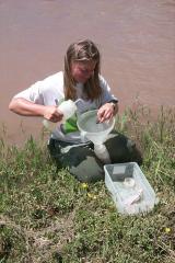
  Visual Estimate

  As part of a field-based rapid periphyton survey developed for use in the Rapid Bioassessment Protocols, a quick visual estimation of algal biomass was developed. This approach uses gridded view buckets to visually estimate macroalgal biomass and microalgal cover. While not as accurate as actual measures of algal biomass, the technique does allow rapid relative estimates of composition and standing crop or biomass.

  Algal Composition

  The composition of the algal assemblage in stream periphyton can provide information about the physical and chemical environment. Unlike simple grab samples of water, the assemblage of algae integrate water quality conditions over long periods of time. Each taxon has specific optima for the wide variety of physical and chemical conditions to which periphyton are exposed, including sensitivities or tolerance to nutrients, acidity, temperature, oxygen, silt, and other variables. The average environmental conditions influence which taxa survive and thrive in a stream. As a result, a great deal of environmental information can be inferred from which algae are found in the periphyton, including nutrient conditions. The composition of algae is usually determined with microscopy, and most taxa can be identified to species by well-trained taxonomists. A rapid visual estimate of rough benthic algal composition has also been developed.

  Microscopy

  Unfiltered periphyton samples collected from the stream should be preserved. The preferred preservative is Lugol’s solution, but other optional preservatives include 2% M3 fixative, 4% buffered formalin, or 2% glutaraldehyde. The sample is typically homogenized with a tissue homogenizer and placed into a specific cell for viewing of large algal taxa (e.g., Palmer-Maloney or Sedgwick-Rafter cells). These can be enumerated a number of ways, but it can be difficult to enumerate colonial or filamentous individuals, and magnification is limited for these sample cells. Sedimentation chambers can also be used for identifying smaller cells if inverted microscopes are available. In this approach, a known subsample of the homogenized sample is placed into a sedimentation chamber, where the algae settle. The chamber is then placed on an inverted microscope, where greater magnification can be used to identify taxa. For diatom analysis, it is necessary to remove organic matter that might otherwise interfere with identification. This can be done with combustion or chemical oxidation of subsamples, followed by slide mounting with a suitable highly refractive medium to make permanent slides. Compound microscopy at 1000x under oil immersion is then used to identify diatoms to species. From these data, accurate identifications of the resident algal periphyton assemblage can be made. When combined with autecological information for the different algal taxa, a number of inferences about the integrated physical and chemical conditions of a stream or lake can be made.

  Rapid visual estimates

  The rapid visual approach uses gridded view buckets to characterize periphyton assemblages. Very coarse-level taxonomic information can be collected by individuals trained to recognize specific macro-algal taxa. The buckets are placed randomly along transects, and the algal assemblage are identified to specific macroalgal genera or to coarse algal groups (e.g., diatoms or blue-green algae).

  Literature Cited

  APHA. 1999. Standard Methods for the Examination of Water and Wastewater. 20th edition. American Public Health Association, Washington, DC.

  Barbour, M.T., J. Gerritsen, B.D. Snyder, and J.B. Stribling. 1999. Rapid Bioassessment Protocols for Use in Streams and Wadeable Rivers: Periphyton, Benthic Macroinvertebrates and Fish, Second Edition. EPA 841-B99-002. U.S. Environmental Protection Agency, Office of Water, Washington, DC.

  Cambridge, M.L., J.R. How, P.S. Lavery, and M.A. Vanderklift. 2007. Retrospective analysis of epiphyte assemblages in relation to seagrass loss in a eutrophic coastal embayment. Marine Ecology-Progress Series 346:97-107.

  Dodds, W.K. 2002. Freshwater Ecology: Concepts and Environmental Applications. Academic Press, New York.

  Frankovich, T.A. and J.W. Fourqurean. 1997. Seagrass epiphyte loads along a nutrient availability gradient, Florida Bay, USA. Marine Ecology-Progress Series 159:37-50.

  Hauer, F.R. and G.A. Lamberti. 1996. Methods in Stream Ecology. Academic Press, New York.

  Hillebrand, H., C.D. Durselen, D. Kirschtel, U. Pollingher, and T. Zohary. 1999. Biovolume calculation for pelagic and benthic microalgae. Journal of Phycology 35: 403-424.

  Moulton II, S.R., J.G. Kennen, R.M. Goldstein, and J.A. Hambrook, 2002. Revised Protocols for Sampling Algal, Invertebrate, and Fish Communities as Part of the National Water-Quality Assessment Program. U.S. Geological Survey Open-File Report 02-150.

  Peterson, B.J., T.A. Frankovich, and J.C. Zieman. 2007. Response of seagrass epiphyte loading to field manipulations of fertilization, gastropod grazing and leaf turnover rates. Journal of Experimental Marine Biology and Ecology 349(1):61-72.

  Stevenson, R.J. and L.L. Bahls. 1999. Periphyton protocols. In Barbour, M.T., J. Gerritsen, B.D. Snyder, and J.B. Stribling. 1999. Rapid Bioassessment Protocols for Use in Streams and Wadeable Rivers: Periphyton, Benthic Macroinvertebrates and Fish. Second Edition. EPA 841-B99-002. U.S. Environmental Protection Agency, Office of Water, Washington, DC.

  Wetzel, R.G. 2001. Limnology: Lake and River Ecosystems. 3rd edition. Academic Press, New York.

  Wetzel, R.G. and G.E. Likens. 2000. Limnological Analyses. 3rd edition. Springer-Verlag, New York.

• Phosphorus

  Phosphorus is a common limiting nutrient in both marine and freshwater systems (e.g., Elser, 2007). Unlike nitrogen, phosphorus exists in one valence state as the phosphate ion, in freshwater (PO₄³-). Phosphates are classified as orthophosphates (single phosphate ions), condensed phosphates (polyphosphates), and organically bound phosphates. Phosphates occur as dissolved or bound forms – either in organic particles or attached to detritus or inorganic sediment. Phosphine gas (PH₃) is rare. Phosphorus in surface waters comes from a variety of sources. Natural sources include bedrock and precipitation. Common anthropogenic sources include fertilizers and detergents, as well as human waste and food residues.

  Phosphorus is divided into particulate and “dissolved” forms, the latter of which are defined principally based on the method selected. The total phosphorus fractions consist of particulate and “dissolved” fractions, measured from an unfiltered sample. Total fractions include phosphate bound in organic and to inorganic particles. Dissolved fractions are those measured after filtration through a membrane filter. Dissolved organic forms include phospho-lipids, nucleic acids, and ATP.

  Phosphate analysis consists principally of converting the various forms of phosphorus to dissolved orthophosphate (PO₄³-) followed by direct colorimetric measurement. The separation of the different forms is analytically defined, but these have been selected to be consistent with more or less functional phosphorus fractions. The separation of dissolved and particulate fractions has traditionally been through 0.45 µm membrane filters. This distinction is not absolute, but it allows for a relatively precise and replicable standard of measurement. Within the dissolved and total phosphorus fractions, phosphorus is further divided into three principal forms of phosphorus: reactive, acid-hydrolyzable, and organic phosphorus.

  Reactive phosphorus, in both dissolved and particulate fractions, is that phosphorus which reacts with reagents in colorimetric tests without hydrolysis or digestion. While reactive phosphorus is principally orthophosphate, it also includes a small fraction of condensed phosphate, which is hydrolyzed during the analysis.

  Acid hydrolysis is used to convert all dissolved and particulate condensed forms into orthophosphate. Again, this process likely liberates some organically bound phosphorus and may include some of that fraction, but this can be minimized procedurally. This analytical artifact is the basis for calling the fraction “acid-hydrolyzable” rather than “condensed phosphate.”

  Lastly, organic and organically-bound phosphorus is that fraction released only by oxidative digestion. Organic phosphorus also occurs in dissolved and particulate forms.

  Sample Collection

  Filtration for dissolved analysis, if desired, usually occurs during or immediately after sample collection. Samples can be frozen or chemically preserved. Equipment type and lab environment can affect phosphorus analysis, so extra care must be taken. Preparation of equipment used in phosphorus collection and analysis is strict and must be adhered to minimize contamination and sample error.

  Acid Hydrolysis and Digestion

  Digestions are used to estimate the total phosphorus and total organic phosphorus fractions (by subtraction). There are three principal digestion techniques: perchloric, nitric acid-sulfuric acid, and persulfate. Perchloric acid digestion is recommended only for the most difficult samples (e.g., sediments) and is time-consuming and severe. Nitric acid-sulfuric acid digestion is appropriate for most samples. Persulfate digestion is the simplest technique and should be checked against the other two for comparability.

  Acid Hydrolysis

  Acid hydrolysis is used for measuring the acid-hydrolyzable fraction and is defined as the difference between the concentrations in an untreated sample (reactive phosphorus) and one treated with mild acid. It includes condensed phosphates and potentially some organic phosphate compounds. This method involves acidifying a sample with sulfuric and nitric acids followed with gentle boiling. The orthophosphate liberated is then measured using one of the colorimetric methods.

  Perchloric Acid Digestion

  This fairly intense procedure involves acidifying a sample with nitric acid and then digesting the sample in a solution of nitric acid and perchloric acid. This is then neutralized with sodium hydroxide. Orthophosphate is then measured using one of the colorimetric methods.

  Sulfuric Acid-Nitric Acid Digestion

  This method uses a digestion rack much like those used for micro-Kjeldahl nitrogen determination. In this approach, sulfuric and nitric acids are added to a sample and digested. The orthophosphate liberated is then measured using one of the colorimetric methods.

  Persulfate Digestion

  In this approach, persulfate is added to a pH-adjusted sample and boiled for a set period of time. The orthophosphate liberated is then measured using one of the colorimetric methods.

  Colorimetric Methods for Phosphate

  The colorimetric methods are fairly similar and depend principally on the range of concentrations desired. The vanadomolybdophosphoric acid method is used for phosphate concentrations between 1 and 20 mg P/L and the stannous chloride and ascorbic acid methods are used for ranges between 0.01 and 6 mg P/L. Extractions and longer cell paths may improve detection on the lower ranges. Ion chromatography and capillary ion electrophoresis methods can also be used for determining orthophosphate concentrations in undigested samples.

  Vanadomolybdophosphoric Acid Method

  The principle of this test is that ammonium molybdate reacts with orthophosphate under acidic conditions and in the presence of vanadium to form a yellow color, which is proportional to the concentration of phosphate in the sample. This color can then be measured with a colorimeter and the phosphate concentration of the sample estimated. Again, this method is generally recommended over the 1 to 20 mg P/L range.

  Stannous Chloride Method

  In this method, molybdophosphoric acid (formed by the reaction of orthophosphate with ammonium molybdate under acidic conditions) is reduced by stannous chloride to form a blue molybdenum color, which is proportional to the concentration of phosphate in the sample. This color can then be measured with a colorimeter and the phosphate concentration of the sample estimated. With long path cells, this method can measure phosphorus down to 0.007 mg P/L. An extraction step using separation with benzene-isobutanol can increase the sensitivity for low concentration samples.

  Ascorbic Acid Method

  In this method, ammonium molybdate and potassium antimonyl tartrate react with orthophosphate under acidic conditions to form phosphomolybdic acid which is reduced to a blue color solution by ascorbic acid. The blue color formed is proportional to the concentration of phosphate in the sample. This color can then be measured with a colorimeter and the phosphate concentration of the sample estimated. The method is accurate to 0.01 mg P/L with a 5 cm cell path length. An extraction step using separation with solvent can increase the sensitivity for low concentration samples. An automated version of this method exists (APHA 1999; Method 4500- P F), which follows the same principal as the manual method but uses continuous flow analytical machines that automate the process and can be used for analyzing samples in large batches. The automated method is applicable over the range of 0.001 to 10.0 mg P /L. Higher concentrations can be diluted.

  Literature Cited

  APHA. 1999. Standard Methods for the Examination of Water and Wastewater. 20th edition. American Public Health Association, Washington, DC.

  Elser, J.J., M.E.S. Bracken, E.E. Cleland, D.S. Gruner, W.S. Harpole, H. Hillebrand, J.T. Ngai, E.W. Seabloom, J.B. Shurin, and J.E. Smith. 2007. Global analysis of nitrogen and phosphorus limitation of primary producers in freshwater, marine and terrestrial ecosystems. Ecology Letters 10:1135-1142.

  Francoeur, S.N. 2001. Meta-analysis of lotic nutrient amendment experiments: detecting and quantifying subtle responses. Journal of the North American Benthological Society 20:358-368.

  Wetzel, R.G. 2001. Limnology: Lake and River Ecosystems. 3rd edition. Academic Press, New York.

  Wetzel, R.G. and G.E. Likens. 2000. Limnological Analyses. 3rd edition. Springer-Verlag, New York.

• Phytoplankton

  Phytoplankton is the assemblage of autotrophs found in the water column, including diatoms, green algae, cyanobacteria, dinoflagellates, and other algal taxa. The phytoplankton includes single celled as well as colonial and filamentous forms, and it includes both true phytoplankton as well as periphytic algae that have been dislodged from the benthos (tychoplankton), especially in rivers. In waterbodies with sufficient residence time where true phytoplankton can develop (e.g., lakes, estuaries, and large rivers), this assemblage is the focus of sampling for algal response to nutrients and is, therefore, important in nutrient criteria development. There are well established relationships between nutrient loading and phytoplankton biomass in lakes. In rivers, the relationships are often more variable than those for lakes.

  As with periphyton, two basic attributes of phytoplankton are most often sampled: biomass and composition. Biomass is generally measured by filtering phytoplankton and weighing the resultant organic matter, extracting the chlorophyll to provide a relative estimate of algal abundance, or counting the number of algal cells and using a biovolume conversion to estimate biomass. Phytoplankton assemblage composition typically consists of preserving a representative sample of water and identifying the algal taxa to the lowest possible taxonomic level. Both biomass and composition can be measured from the same field samples, which are split into a subsample for biomass and one for assemblage composition.

  Chlorophyll a (analysis discussed below) has become one of the most widely used response variables when determining nutrient impairment. The benefits of chlorophyll a as an indicator are its sensitivity to stressors, such as nutrients, and ease of monitoring. Higher concentrations of chlorophyll a are indicative of algal production, which is responsive to nutrient pollution. A weakness of chlorophyll a as a measure of phytoplankton biomass/production is the variability of cellular chlorophyll content.

  While many phytoplankton species cause harm in the context of eutrophication, others produce toxins, which can have a serious impact on aquatic systems. Harmful algal blooms (HABs) form as the result of proliferation of toxic nuisance algae and can cause a negative impact to natural resources and human health. Recently, there has been a noticeable increase in problems associated with HABs. Impacts of these natural phenomena include human illness (or death) from contaminated seafood, marine mammal and seabird deaths, and extensive fish kills. Of particular concern in freshwaters are cyanotoxins produced by cyanobacteria or blue-green algae. Cyanobacteria are abundant in most surface water when conditions are favorable for algal blooms. Cyanotoxins include neurotoxins, hepatotoxins, and dermatoxins and may cause a wide range of symptoms in humans. Microcystins are known to cause liver and kidney damage and may have severe long-term effects. For more information on HABs, refer to Harmful Algal Blooms.

  The following is a brief review of common methods. Interested readers are encouraged to examine the literature cited for more detailed methodologies and greater background information.

  Sample Collection

  Phytoplankton samples can be collected using quantitative or semi-quantitative methods. Quantitative methods consist of sampling a volume of water, usually with a sampling device that can isolate a known volume at a specific depth (e.g., Van Dorn, Niskin, Nansen, or Kemmerer Bottle). Another option is to use a long, straight tubular sampler, which allows the collection of a depth integrated sample, essentially a “core” of the water column that collects plankton over a range of depths.

  Algal Biomass

  Algal biomass refers to the mass of algal material within the phytoplankton. It can be measured gravimetrically (weighed), using chlorophyll extractions, or by converting cell count data to mass using biovolume conversions. Gravimetric measures rely on weighing the amount or organic matter within the phytoplankton. As it is generally prohibitive to separate algal and non-algal material for routine analysis, the mass (usually the mass after combustion called ash-free dry mass [AFDM]) can include substantial non-algal material, although this is generally more severe in lotic than lentic systems. Some people use AFDM to chlorophyll ratios to look at the proportion of non-algal material, but this is only an approximation. The content of chlorophyll per cell varies with a number of factors: including species, nutrient conditions, light condition, and temperature. Therefore, chlorophyll is not a direct measure of biomass. However, it has long been used as a relative measure of algal abundance. Cell biovolumes vary by taxa, their shapes, and a number of other factors affecting cellular composition. However, if quantitative genus or species level data are collected, then biovolume can generally be estimated by applying shape specific geometric volume conversions.

  Ash-free dry mass (AFDM)

  A subsample of the original phytoplankton sample is either weighed in pre-combusted and pre-weighed crucibles or weighed following filtration through appropriate pre-weighed and pre-combusted glass fiber filters (0.5-0.7 µm pore size). Crucibles and filters are then dried, weighed for dry mass, and then combusted to remove all organic matter (e.g., 500ºC) and re-weighed to estimate AFDM. Samples for AFDM can be field filtered or brought to the lab for processing there. Sample preservation for AFDM is not straightforward, but samples should be handled to limit respiratory loss of organic matter [e.g., placed on ice and frozen (-20 to -60°C) if there will be a delay in processing]. Consult the specific methods for more on sample preservation. Values are expressed as grams AFDM per unit volume.

  Pigment analysis

  A subsample of the phytoplankton sample is usually filtered onto glass fiber filters (0.5-0.7 µm pore size) and used for pigment analysis as an indicator of algal biomass. On average, chlorophyll constitutes 1.5 percent of the AFDM of algae, but the ratio of chlorophyll to cell biomass varies by taxa, so biomass estimates using this technique should be considered relative. The composition of photosynthetic pigments also varies by algal taxa, but chlorophyll a is the principal pigment used because it is the most common and abundant. Chlorophylls b and c and the carotenoids absorb light at different wavelengths and can be quantified as well, if desired.

  Chlorophyll a degrades into different phaeopigments that absorb at the same wavelength as chlorophyll a. For this reason, chlorophyll concentration is usually measured in a sample after extraction, acidified to convert all the chlorophyll to phaeopigments, remeasured, and chlorophyll a concentration is determined by the difference. Chlorophyll a is historically and most commonly measured using spectrophotometry, although fluorometry is more sensitive and becoming more commonly used.
  

  Chlorophyll and other photopigments must be extracted from algae to quantify biomass using pigment analysis. It is best to work in low light to avoid degradation. While a variety of extraction solvents exist, alkaline aqueous acetone is still the standard recommended method. Algae retained on glass fiber filters (0.5-0.7 µm pore size) are typically ground in aqueous acetone, allowed to extract for a period of time under refrigeration in the dark, and the ground filter solution is centrifuged to separate the filter from the pigments. Pigments are then decanted and measured directly either with spectrophotometry or fluorometry. The flourometric method is usually standardized using spectrophotometric measurement of a chlorophyll extract and while fluorometry is more sensitive it should give comparable estimates. Consult an appropriate methods source for details on the use of either of these detection methods, including appropriate detectors, wavelengths, etc.

  Preservation of samples for chlorophyll is important. Filtration should occur as soon as possible and chlorophyll should be extracted from filters as soon as possible. Field filtration is ideal. Addition of magnesium carbonate either to the sample solution or on top of the filter after filtration has been advocated to reduce acidity, since acidity degrades chlorophyll. Filters that will not be analyzed immediately, should be folded in half, placed into labeled dark containers (e.g., wrapped in aluminum foil), and placed on ice or immediately frozen. Pigment samples may be frozen for a few days (at -20 to -60°C), but should be analyzed as soon as possible, since degradation of chlorophyll does occur.

  Biovolume

  Biovolume is determined by multiplying the number of each taxon identified in a sample by the average biovolume of that taxon, calculated using equations of geometric shapes most approximating the shape of each taxon, and summing these values across all the taxa in a sample. Equations for many different taxa have already been developed or general equations may be applied. This approach obviously requires more effort, since individual taxa must not only be counted but average dimensions may calculated for each as well (average of 20 individuals is recommended, APHA 1999). This method does, however, offer one of the more accurate measures of live algal biomass.

  Algal Composition

  The composition of the algal assemblage of phytoplankton can provide information about the physical and chemical environment. Unlike simple grab samples of water, the assemblages of algae integrate water quality conditions over long periods of time. Each taxon has specific optima for the wide variety of physical and chemical conditions to which phytoplankton are exposed, including sensitivities or tolerance to nutrients, acidity, temperature, oxygen, silt, etc. The average environmental conditions influence which taxa survive and thrive. As a result, a great deal of environmental information, including nutrient conditions, can be inferred from which algae are found in the phytoplankton. This approach is applied by paleolimnologists, who identify the diatoms found in sedimentary strata of lakes to infer historical, even ancient, lake environmental conditions based on this principle. The composition of algae is usually determined with microscopy, and most taxa can be identified to species by well-trained taxonomists.

  Microscopy

  Unfiltered phytplankton samples should be preserved. The preferred preservative is Lugol’s solution, but other optional preservatives include 2% M3 fixative, 4% buffered formalin, or 2% glutaraldehyde. Phytoplankton samples containing macroalgae can be homogenized with a tissue homogenizer and placed into a specific cell for viewing larger algal taxa [e.g., Sedgwick-Rafter (up to 200x) or Palmer-Maloney (up to 500x) cells]. These can be enumerated a number of ways, but it can be difficult to enumerate colonial or filamentous individuals. Magnification is limited with these cells, so microphytoplankton often cannot be identified accurately. Sedimentation chambers and inverted microscopes(500-600x) are ideal for identifying large and smaller cells together. In this approach, a known subsample of the homogenized sample is placed into a sedimentation chamber, where the algae settle. The chamber is then placed on an inverted microscope, where higher objectives may be used. Ocular grids may improve counting efficiency. For the highest magnification (1000x), upright microscopes with oil immersion lenses are required. These are typically used for small diatom analysis. For diatom analysis, it is necessary to remove organic matter that might otherwise interfere with identifying diatoms. This can be done with combustion or chemical oxidation of subsamples, followed by slide mounting with a suitable highly refractive medium to make permanent slides. Other options include membrane filtration followed by clearing of the membranes. Compound microscopy at 1000x under oil immersion is then used to identify diatoms to species. Again, use of ocular grids may increase counting efficiency considerably. From these samples, accurate identification of the resident phytoplankton assemblage can be made. When combined with autecological information for the different algal taxa, a number of inferences about the integrated physical and chemical conditions of a lake can be made.

  Remote Sensing

  Phytoplankton can also be assessed via remote sensing of chlorophyll a. Ocean color satellites are capable of detecting optical components, such as chlorophyll a, and their respective concentrations in the water column according to the wavelengths of light they individually reflect back to the sensor. The sensor measures the remotely sensed chlorophyll a (chlorophyll_RSa) signal by detecting the water leaving radiance in selected wavelengths of light per unit area. The signal read by the sensor is then used to derive quantitative information on the substances in the water and their concentrations in the near­ surface layers.

  Literature Cited

  APHA. 1999. Standard Methods for the Examination of Water and Wastewater. 20th edition. American Public Health Association, Washington, DC.

  Boyer, J.N., C.R. Kelble, P.B. Ortner, and D.T. Rudnick. 2009. Phytoplankton bloom status: Chlorophyll a biomass as an indicator of water quality condition in the southern estuaries of Florida, USA. Ecological Indicators 9 (6, Supplement 1):S56-S67.

  Hillebrand, H., C.D. Durselen, D. Kirschtel, U. Pollingher, and T. Zohary. 1999. Biovolume calculation for pelagic and benthic microalgae. Journal of Phycology 35: 403-424.

  USEPA. 2012. Technical Support Document for U.S. EPA’s Proposed Rule for Numeric Nutrient Criteria, Volume 2 Coastal Waters. U.S. Environmental Protection Agency, Washington, DC.

  USEPA. 2012. Cyanobacteria and Cyanotoxins: Information for Drinking Water Systems. EPA-810F11001. U.S. Environmental Protection Agency, Washington, DC.

  Wetzel, R.G. 2001. Limnology: Lake and River Ecosystems. 3rd edition. Academic Press, New York.

  Wetzel, R.G. and G.E. Likens. 2000. Limnological Analyses. 3rd edition. Springer-Verlag, New York.

• Additional Information

  ASTM Water Testing Standards Exit

  Aquatic Informatics Resources Exit - Aquatic Informatics, Inc. has compiled a series of resources relating to water quality monitoring including an ebook, white papers, webinars, and case studies.

  EPA Clean Water Act Analytical Methods - EPA publishes laboratory analytical methods or test procedures that are used by industries and municipalities to analyze environmental samples that are required by regulations under the authority of the Clean Water Act.

  EPA Wetlands Modules - EPA prepared these modules to give states and tribes "state-of-the-science" information that will help them develop biological assessment methods to evaluate both the overall ecological condition of wetlands and nutrient enrichment.

  National Environmental Methods Index (NEMI) - A free, searchable clearinghouse of methods and procedures for both regulatory and non-regulatory monitoring purposes for water, sediment, air, and tissues.

  USGS Water Quality Methods and Techniques - USGS provides links to compiled information on water quality sampling methods.

  USGS Field Guide for Collecting and Processing Stream - Water Samples for the National Water-Quality Assessment Program - The USGS National Water-Quality Assessment (NAWQA) program includes extensive data-collection efforts to assess the quality of the United States’ streams. These studies require analyses of stream samples for major ions, nutrients, sediments, and organic contaminants. This field guide describes the standard procedures for collecting and processing the previously mentioned samples, as well as field analyses of conductivity, pH, alkalinity, and dissolved oxygen.

Statistical Tools

Fact sheets on statistical information commonly used in nutrient criteria development and links to other statistical resources.

• Change-Point Analysis

  Change-point analysis is a method for identifying thresholds in relationships between two variables.
  Change-Point Analysis Fact Sheet

• Correlation

  Correlation is a measure of the strength of a relationship between two variables.
  Correlation Fact Sheet

• Loess or Lowess

  Loess stands for locally estimated scatterplot smoothing (lowess stands for locally weighted scatterplot smoothing) and is one of many non-parametric regression techniques.
  Loess or Lowess Fact Sheet

• Regression

  Regression is one of the most common statistical modeling tools used, regression is a technique that treats one variable as a function of another.
  Regression Fact Sheet

• Conditional Probability

  A conditional probability is the probability of an event occurring when some other event has occurred.
  Conditional Probability Fact Sheet

• Classification

  Classification, in the nutrient criteria process, is the process of identifying groups of sites that have comparable characteristics and for which comparable nutrient behavior is expected.
  Classification Fact Sheet

• Weighted Averaging

  Weighted averaging is a method for computing an average where some values receive greater weight than others.
  Weighted Averaging Fact Sheet

• Links to Other Statistical Resources

  The following links exit the site Exit

  Statistics Resources

  • List of webpages that Perform Statistical Calculations - Exhaustive list of statistical test.
  • Vassar College “VassarStats” page - Online calculator of statistical functions.
  • College of St. Benedict, Statistics Calculators - Online calculator of statistical functions.
  • GraphPad QuickCalcs - Online Calculators For Scientists to Analyze, Graph, and Organize Data.

  Software

  • R - Widely used free software environment for statistical computing and graphics. It compiles and runs on a wide variety of UNIX platforms, Windows and MacOS.
  • R Studio - Provides a graphical interface for use with R.
  • Free Statistical Packages (BUGS, R, STATS) - Free software that will run different statistical tests.
  • University of Minnesota - Arc Software - A package for regression analysis designed as a companion to the book Applied Regression Including Regression and Graphics by R.D. Cook and S. Weisberg.
  • Statistical Analysis Tools - Analysis programs, power analysis, stats tables (t distribution, chi square, normal distribution, etc.); describes univariate data, curve fitting, and distribution-free tests.

  Open Source Statistics Training

  • Coursera homepage and Coursera Statistical Topics - Offers over 700 free courses on a variety of topics; with over 50 participating universities offering statistical courses.
    • Coursera offers a data science specialization in a 9 part series that may be of interest.
  • Rice University Virtual Statistics lab - Stats tools and case studies, demonstrations, and books for background information and resources.
    • Rice University Online Statistics Book.
  • Carnegie Mellon University - Through its Open Leaning Initiative offers courses in Statistical Reasoning and Probability and Statistics among other courses.

Model Descriptions

Brief descriptions of selected models commonly used in nutrient water quality modeling are included below, and the introductory table shows them sorted by model type: watershed model, hydrodynamic model, water quality model, and nutrient BMP (best management practice) model. These models are commonly used in concert with each other such that a watershed model may be linked to a hydrodyamic model on the same project. Thus, the examples included in the Models in Action section for each model will frequently include more than one model.

For help determining which model or models are best suited for your needs consider the Water Environment Research Foundation’s (WERF) LINK1T11 software Exit.

The types of models commonly used in nutrient water quality modeling include:

Water Quality Models

• Describe changes that occur to contaminants (e.g., eutrophication models describe nutrient cycles; growth of algae; and production and consumption of dissolved oxygen)

Watershed Models

• Describe hydrologic mechanisms (e.g., flow)
• Describe delivery of contaminants from the watershed to a stream, river, lake, or estuary (e.g., temperature, total nitrogen, total phosphorus, total suspended solids, dissolved oxygen, biochemical oxygen demand)

Hydrodynamic Models

• Describe water movement (e.g., volume, velocity, direction); can describe the water movement in one, two, or three dimensions over varying time periods
• Simulate corresponding changes in properties (e.g., temperature and salinity)

Nutrient BMP Models

• Aid in the selection of Nutrient BMPs and forecasting of nutrient removal effectiveness and cost

Note some models fit in more than one category.

Model	Water Quality Model	Watershed Tools/Models	Hydrodynamic Model	Nutrient BMP Model
AQUATOX
BASINS
BATHTUB
BMP-DSS
CE-QUAL-W2
ECOMSED
EFDC
EPD-RIV1
HSPF
LSPC
QUAL2K
QUAL2KW
SPARROW
SUSTAIN
SWAT
SWMM
WAM
WARMF
WASP

• AQUATOX

  AQUATOX Model Version 3.1

  Overview

  AQUATOX is an ecosystem model that simulates the transfer of biomass and chemicals from one compartment of the ecosystem to another by simultaneously computing important chemical and biological processes over time. It can predict the fate of nutrient and organic chemical pollutants in aquatic ecosystems and their direct and indirect effects on the resident organisms, such as fish, invertebrates, and aquatic plants. Because AQUATOX models the interaction between biota and their environment, the model can be used to help establish the cause and effect relationships between chemical water quality, the physical environment, and aquatic life.

  AQUATOX is well suited for analysis of streams and lakes under stress from nutrient enrichment, such as nuisance algal blooms. It is one of the few models that can simulate impacts to periphyton (attached algae) response to nutrients, grazing, and flow. In addition, the model can simulate multiple types of phytoplankton and their successive blooms throughout the season in lakes and reservoirs and the vertical stratification that occurs in such water bodies.

  AQUATOX is a valuable tool for ecologists, biologists, water quality modelers, and anyone involved in performing ecological risk assessments for aquatic ecosystems. Potential applications would include development or evaluation of water quality criteria for nutrients, total maximum daily loads (TMDLs), and analysis of management alternatives.

  What’s new in this version?

  AQUATOX Release 3.1 Plus includes the following enhancements:

  • The option to model nutrient limitation in plants is based on internal rather than external nutrients. This allows for luxury uptake of nutrients during high-nutrient periods and expenditure of nutrient stores during lower-nutrient periods. Concentrations and derivative rates may be output from these new internal, nutrient-state variables as well as the nutrient-to-organism ratio for each plant. This option should improve the prediction of the timing and duration of algal blooms.
  • Sinking of plants and suspended detritus is now affected by the salinity and therefore the density of water in non-estuary segments.
  • There are new outputs for net primary productivity, pelagic invertebrate biomass, benthic invertebrate biomass, and fish biomass.
  • There is now the capability to load and save observed data to a file to move from one study to another.
  • The model has been significantly optimized for loading and saving of very large aps or als files.
  • For moving water (streams and rivers), the average water temperature must drop below 0 degrees C before ice cover is assumed.  Additionally information on the enhancements included in
    Additional information on the enhancements included in AQUATOX Release 3.1 Plus

  Model in action

  Nutrient and eutrophication analysis
  AQUATOX was applied to a dataset from Walker Branch, a woodland stream in Tennessee. Researchers calibrated the model with experimental data and manipulated nutrients, light, and grazer (snail) populations. They verified the model by applying it to independent data on the same stream, with good agreement between observed values and model predictions. Results showed that control of the temporal pattern and magnitude of periphyton in this stream was dependent on nitrogen and phosphorus concentrations; riparian vegetation (which affects light reaching the stream); grazing by snails; and water velocity. The study demonstrates the necessity to model grazers in order to accurately simulate periphyton
  Modeling periphyton with AQUATOX

  How to access the model

  Download the AQUATOX model

  More information

  Model description
  AQUATOX validation reports and publications

• BASINS (Best Management Science Integrating Point and Nonpoint Sources)

  BASINS Model Version 4.1

  Overview

  BASINS is a multipurpose environmental analysis system for use by regional, state, and local agencies in performing watershed- and water quality-based studies. BASINS makes watershed and water quality studies easier by bringing together key data (e.g., elevations and observed data stations) and analytical components in one tool.

  It was developed by EPA's Office of Water to address three objectives:

  • To facilitate examination of environmental information
  • To support analysis of environmental systems
  • To provide a framework for examining management alternatives.

  BASINS allows users to efficiently access national environmental information, incorporate local site-specific data, apply assessment and planning tools, and run a variety of proven, robust nonpoint loading and water quality models. A geographic information system (GIS) provides the integrating framework for BASINS, which organizes spatial information so it can be displayed as maps, tables, or graphics. BASINS is a useful tool for those interested in watershed management, development of total maximum daily loads (TMDLs), coastal zone management, nonpoint source programs, water quality modeling, and National Pollutant Discharge Elimination System (NDPES) permitting.

  What’s new in this version?

  BASINS 4.1 is the most current model release. Improvements to the model include:

  • BASINS 4.1 is built upon the latest stable release of the non-proprietary, open-source MapWindow GIS. The new MapWindow interface has changed in appearance from BASINS 4.0, but the main functions remain the same.
  • The BASINS automatic watershed delineation tools have been updated to use TauDEM (Terrain Analysis Using Digital Elevation Models) version 5 from Utah State University. TauDEM is a software program that delineates watershed boundaries from topographic information such as elevation grids, slope, and stream flow direction.
  • Beginning with BASINS 4.1, two of the main utilities, GenScn and WDMUtil, are available as separate downloads. However, most of the functionality of GenScn and WDMUtil is now included in the core BASINS user interface, making the separate programs unnecessary for most users.
  • BASINS 4.1 includes DFLOW, a tool to estimate design stream flows for use in water quality studies.
  • The BASINS 4.1 User Manual has been updated to reflect the current software.
  • BASINS 4.1 is verified for 64-bit and Windows 8 compatibility.
    What has changed between BASINS 4.0 and 4.1?

  Model in action

  EPA's Support of Nutrient Criteria for Florida

  EPA has used and supported the use of several models in the development of numeric nutrient criteria.  As part of its technical support and collaboration with the state of Florida to develop numeric nutrient criteria for estuaries, EPA proposed using watershed models (LSPC) coupled with estuarine hydrodynamic and water quality simulation models (EFDC and WASP) to address the physical, chemical, and biological processes influencing watershed nutrient delivery and nutrient-related responses. BASINS was used to obtain the GIS data files required to set-up and calibrate the LSPC models, which represented the hydrological and water quality conditions in the watersheds. Files downloaded using BASINS include the digital elevation model, National Hydrography Dataset, and United States Geological Survey station locations.  Since then, Florida has incorporated some of these approaches in the development of the numeric nutrient criteria adopted for estuaries.
  Florida's nutrient criteria for estuaries (Refer to technical support document for estuaries)

  How to access the model

  Download BASINS model

  More information

  General information about BASINS

  User information and guidance
• BATHTUB

  Overview

  The BATHTUB model is designed to facilitate application of empirical eutrophication models to morphometrically complex reservoirs. The program performs water and nutrient balance calculations in a steady-state, spatially segmented hydraulic network that accounts for advective transport, diffusive transport, and nutrient sedimentation. Eutrophication-related water quality conditions (expressed in terms of total phosphorus, total nitrogen, chlorophyll a, transparency, organic nitrogen, nonortho-phosphorus, and hypolimnetic oxygen depletion rate) are predicted using empirical relationships previously developed and tested for reservoir applications.

  To reflect data limitations or other sources of uncertainty, key inputs to the model can be specified in probabilistic terms (mean and coefficient of variation (CV)). Outputs are expressed in terms of a mean value and CV for each mass balance term and response variable. Output CVs are based upon a first-order error analysis, which accounts for input variable uncertainty and inherent model error.

  Applications of BATHTUB are limited to steady-state evaluations of relations between nutrient loading, transparency and hydrology, and eutrophication responses. Short-term responses and effects related to structural modifications or responses to variables other than nutrients cannot be explicitly evaluated.

  Model in action

  Grand Lake Saint Marys BATHTUB Model

  A BATHTUB model was developed by Ohio Environmental Protection Agency for Grand Lake Saint Marys to assess the impacts of reducing total phosphorus and nitrate loads to the lake.
  TMDL Development for the Beaver Creek and Grand Lake St. Mary' (PDF) (18 pp, 367 K)

  Lake Champlain BATHTUB Model Report

  A BATHTUB model was used to determine watershed point and nonpoint total phosphorous (TP) load reductions required to meet in-lake TP criteria established for each of the 13 lake segments of Lake Champlain as part of a 2002 TMDL.
  Lake Champlain Phosphorus TMDL

  How to access the model

  Download BATHTUB model

  More information

  BATHTUB Fact Sheet (PDF) (2 pp, 117 K)

• BMP-DSS (Best Management Practice Decision Support System)

  Overview

  The Best Management Practice Decision Support System (BMP-DSS) evaluates potential watershed management opportunities by quantifying potential best management practice (BMP) benefits and their costs. The modeling system supports watershed hydrologic and water quality analysis, simulates a variety stormwater BMPs, and optimizes selection and placement of BMPs. The system helps planners to determine which solution alternatives provide the greatest benefit for achieving management targets while balancing costs.

  The proper selection and placement of BMPs is a critical part of the stormwater planning effort. Established urban and newly developing areas must establish cost effective means for restoring existing sites, minimizing impacts to new sites, and provide general site planning for future growth. BMP-DSS supports watershed hydrologic and water quality analysis, simulation of various innovative BMPs, and selection/placement optimization of suitable BMPs that will achieve project goals, as defined by a user. This system helps planners determine which alternatives will yield the greatest benefit by automatically assessing several key site-specific factors.

  BMP-DSS is a process based simulation model for BMPs, it provides a technique that is sensitive to local climate and rainfall patterns as well as BMP size, design, and relative placement on the site. The system incorporates a meta-heuristic optimization technique to find the most cost-effective BMP placement and implementation plan that best satisfies a controlled target and fits within a fixed cost budget.

  Model in action

  Prince George’s County, Maryland BMP Evaluation

  The BMP-DSS model was used to assist Prince George’s County, Maryland to evaluate BMPs in a green highway project located in the Anacostia River watershed. The area is highly urbanized and is located within the District of Columbia. Several BMPs, such as bioretention, green roof, porous paving, and rain barrels were proposed to minimize runoff, improve water quality, and provide water reuse opportunities. The modeling system was used to identify and evaluate various alternatives to determine the most cost-effective types and combinations of BMPs that best minimize the frequency and size of runoff events thereby also reducing the magnitude and frequency of combined sewer overflows to the Anacostia River.
  BMP decision support system for evaluating stormwater alternatives

  How to access the model

  For more information, email (nutrient.criteria@tetratech.com).

• CE-QUAL-W2

  Overview

  CE-QUAL-W2 is a two-dimensional (longitudinal/vertical) hydrodynamic and water quality model that has been successfully applied to over 400 systems throughout the United States and internationally.

  Relevant hydrodynamic/transport capabilities include dynamic adjustment of the timestep to help ensure numerical stability, variable vertical/longitudinal grid spacing, wetting/drying, multiple point/nonpoint sources, and a higher-order numerical transport scheme (QUICKEST/ULTIMATE) that reduces numerical diffusion and eliminates physically unrealistic over/undershoots. Geometrically complex waterbodies can be represented through multiple branches and cells. Multiple inflows and outflows to the waterbody are represented through point/nonpoint sources, branches, precipitation, and other methods. Tools for modeling hydraulic structures, such as spillways and pipes are available. Output from the model provides options for detailed and convenient analyses.

  Relevant water quality capabilities include any number of generic constituents that could include a conservative tracer, and/or water age, and/or coliform bacteria groups. These generic constituents are defined by a settling velocity, and/or a 0-order decay rate, and/or a 1st order decay rate, and/or an Arrhenius temperature rate multiplier. The model can also simulate any number of phytoplankton groups; any number of carbonaceous biochemical oxygen demand (CBOD) groups; and any number of inorganic suspended solids groups, phosphate, ammonium, nitrate/nitrite, dissolved silica, particulate biogenic silica, dissolved iron, dissolved oxygen, total inorganic carbon, and alkalinity. The model also has the capability to internally compute and output derived variables such as pH, total organic carbon (TOC), particulate organic carbon (POC), and dissolved organic phosphorus for comparison to measured observed data. However, several water quality processes are not simulated including zooplankton, macrophytes, and a dynamic sediment oxygen demand.

  What’s new in this version?

  Enhancements of Version 3.7 include:

  • The model is improved to handle river flow regimes.
  • There is a new bathymetry file input format in comma delimited format (csv) that is easily developed using Microsoft Excel. This simplifies setting up the initial grid and debugging it.
  • Temperature and dissolved oxygen habitat volumes are now computed within the model for user-specified fish species.
  • There is a new automatic selection of a withdrawal port algorithm that will select the elevation of the withdrawal necessary to meet temperature targets including splitting flows between outlets to reach a target temperature.
  • Since each BOD group can have a different BOD-P, BOD-C and BOD-N stoichiometric equivalent, it was necessary to add to the model new state variables, BOD-P, BOD-N, and BOD-C that allowed for time variable inputs of BOD-P, BOD-C and BOD-N from a point or non-point source.
  • Environmental performance criteria were developed to evaluate time and volume averages over the system of state variables chosen for analysis. This is an easy method for looking at water quality differences between model runs.
  • The model now has a module for adding dissolved oxygen, such as hypolimnetic aeration, to specific locations based on a dynamic dissolved oxygen probe monitoring the dissolved oxygen levels.
  • The model has a dynamic pipe algorithm allowing a pipe to be turned ON or OFF over time, as if a gate was closed.
  • The model also has a dynamic pump algorithm that allows the model user to set dynamic parameters for the water level control over time. This is very useful in setting rule curves for operation of the reservoir water levels over time.
  • The maximum time step can now be set to interpolate its value over time rather than suddenly changing the maximum time step. This allows for a smoother change in the model time step.
  • The computation of the temperature at which ice freezes has been adjusted to account for salt water impacts.
  • New model output includes volume weighted averages of eutrophication water quality variables as a function of segment and for only surface conditions as specified by the model user. Other new output includes output of flows, concentrations, and temperatures from a segment for all individual withdrawals.

  Model in action

  Klamath River System TMDL Development

  To support TMDL development for the Klamath River system, an integrated receiving water hydrodynamic and water quality modeling system was used that consisted of EFDC, CE-QUAL-W2, and RMA. CE-QUAL-W2 was used to model several reservoirs that were part of the Klamath River system.

  • Review of Revised Klamath River Total Maximum Daily Load Models from Link River Dam to Keno Dam, Oregon (PDF) (38 pp, 1 MB)
  • Klamath River Model for TMDL Development (PDF) (163 pp, 7 MB)

  Summit Water Distribution Company Environmental Assessment

  U.S. Department of the Interior used CE-QUAL-W2 as part of the Environmental Assessment of a proposal for Summit Water Distribution Company to build and operate facilities to deliver water to the Park City/Snyderville Basin area in Utah.

  • Final Environmental Assessment East Canyon Reservoir Water Intake Structure and Finding of No Significant Impact
  • Water Quality Modeling Using CE-QUAL-W2 (PDF) (17 pp, 2 MB)

  How to access the model

  Download the CE-QUAL-W2 model

• ECOMSED (Estuary and Coastal Ocean Model with Sediment Transport)

  Overview

  ECOMSED is a three-dimensional hydrodynamic and sediment transport model that can be used to simulate conditions in rivers, lakes, and estuaries. The hydrodynamic module solves the conservation of mass and momentum equations with a 2.5-level turbulent closure scheme on a curvilinear orthogonal grid in horizontal plane and σ-coordinate in the vertical direction. Water circulation, salinity, and temperature are obtained from the hydrodynamic module. The sediment transport module computes the sediment settling and resuspension processes for both cohesive and noncohesive sediments under the impact of waves and currents.

  The hydrodynamic component of ECOMSED is based on the 1980s Princeton Ocean Model, which has been tested and applied by various users. In the mid-1990s, concepts for sediment resuspension and settling developed by W. Lick at the University of California, Santa Barbara were incorporated within the ECOM modeling framework. The ECOMSED model was developed, and is maintained, by HydroQual.

  Model in action

  ECOMSED has been applied to waterbodies including Chesapeake Bay, New York Bight, Delaware Bay, Delaware River, Gulf Stream Region, Massachusetts Bay, Georges Bank, the Oregon Continental Shelf, New York Harbor, and Onondaga Lake. Some examples include:

  • Executive Summary: Upper Mississippi River – Lake Pepin Water Quality Model (PDF) (4 pp, 75 K)
  • Murderkill River TMDL Report – Delaware Department of Natural Resources and Environmental Control (PDF) (140 pp, 23 MB)

  How to access the model

  ECOMSED is available for download to interested users by registering through HydroQual's website. The software will be distributed only to registered users so that HydroQual can provide upgrades, “bug fixes,” and other information to users without delay.

  More information

  For more information about the model, visit

  • HydroQual’s website
  • Environmental Hydrodynamics
• EFDC (Environmental Fluid Dynamics Code)

  Overview

  EFDC is a state-of-the-art hydrodynamic model that can be used to simulate aquatic systems in one, two, and three dimensions. It has evolved over several decades to become one of the most widely used and technically defensible hydrodynamic models in the world. EFDC uses stretched or sigma vertical coordinates and Cartesian or curvilinear, orthogonal horizontal coordinates to represent the physical characteristics of a waterbody. It solves three-dimensional, vertically hydrostatic, free surface, turbulent averaged equations of motion for a variable-density fluid. Dynamically-coupled transport equations for turbulent kinetic energy, turbulent length scale, salinity, and temperature are also solved. The EFDC model allows for drying and wetting in shallow areas by a mass conservation scheme. A preprocessor is being developed to facilitate the setup and application of EFDC for a wide range of applications.

  Model in action

  EFDC Application for the Neuse River Estuary, North Carolina

  The Neuse River Estuary was included on North Carolina’s 303(d) list for nutrients and was scheduled for TMDL development. Water quality targets were ultimately based on a chlorophyll a concentration of 40 mg/L.

  How to access the model

  Download the EFDC model

  More information

  More information about the EFDC model

• EPD-RIV1 (One Dimensional Riverine Hydrodynamic and Water Quality Model)

  Overview

  The EPD-RIV1 package contains user-friendly programs designed to model one-dimensional waterbodies with special emphasis on the needs of regulatory decision making, including TMDLs and conventional wasteload allocations. Initially based on CE-QUAL-RIV1 (developed by the U.S. Army Engineers Waterways Experiment Station), EPD-RIV1 now contains both hydro-dynamic and water quality models, is managed by a robust preprocessor, and is supported by a capable post processor. Each component is integrated with the Water Resources Database, which is also a standalone part of the tool kit. For complex one-dimensional river systems with issues that do not involve sediment transport, toxics, or metals, EPD-RIV1 would be the model of choice. It uses state-of-the-art solution routines and provides defensible results for regulatory decision making.

  Model in action

  Savannah Harbor Dissolved Oxygen TMDL

  EPD-RIV1 was used as part of the Savannah Harbor TMDL for Dissolved Oxygen (2010) to transport oxygen demanding substances from the upper watershed to the Harbor Model (EFDC and WASP).
  Report: Savannah Harbor TMDL for Dissolved Oxygen (2010) (PDF) (39 pp, 1 MB)

  How to access the model

  Download the EPD-RIV1 model

• HSPF (Hydrological Simulation Program – FORTRAN)

  Overview

  HSPF is a comprehensive package for simulation of watershed hydrology and water quality for both conventional and toxic organic pollutants. HSPF incorporates watershed-scale agricultural runoff model and nonpoint source (NPS) models into a basin-scale analysis framework that includes fate and transport in one dimensional stream channels. It is a comprehensive model of watershed hydrology and water quality that allows the integrated simulation of land and soil contaminant runoff processes with in-stream hydraulic and sediment-chemical interactions. The result of this simulation is a time history of the runoff flow rate, sediment load, and nutrient and pesticide concentrations, along with a time history of water quantity and quality at any point in a watershed. HSPF simulates three sediment types (sand, silt, and clay) in addition to a single organic chemical and transformation products of that chemical.

  HSPF uses continuous rainfall and other meteorologic records to compute streamflow hydrographs and pollutographs. HSPF simulates interception soil moisture, surface runoff, interflow, base flow, snowpack depth and water content, snowmelt, evapotranspiration, ground-water recharge, dissolved oxygen, biochemical oxygen demand (BOD), temperature, pesticides, conservatives, fecal coliforms, sediment detachment and transport, sediment routing by particle size, channel routing, reservoir routing, constituent routing, pH, ammonia, nitrate-nitrite, organic nitrogen, orthophosphate, organic phosphorus, phytoplankton, and zooplankton. The program can simulate one or many pervious or impervious unit areas discharging to one or many river reaches or reservoirs. Frequency-duration analysis can be done for any time series. HSPF is generally used to assess the effects of land-use change, reservoir operations, point or nonpoint source treatment alternatives, flow diversions, and others factors. Programs, available separately, support data preprocessing and postprocessing for statistical and graphical analysis of data saved to the Watershed Data Management (WDM) file.

  Potential applications and uses of the model include:

  • Flood control planning and operations
  • Hydropower studies
  • River basin and watershed planning
  • Storm drainage analyses
  • Water quality planning and management
  • Point and nonpoint source pollution analyses
  • Soil erosion and sediment transport studies
  • Evaluation of urban and agricultural best management practices
  • Fate, transport, exposure assessment, and control of pesticides, nutrients, and toxic substances analyses
  • Time-series data storage, analysis, and display

  What’s new in this version?

  Corrections and improvements to prior versions include:

  • Atmospheric deposition can be input to most of the water quality constituents in HSPF.
  • The soil nutrient calculations in PERLND have undergone major modifications to facilitate modeling of agricultural practices and forest areas.
  • Water categories can be defined and tracked in streams and rivers.
  • The Special Actions (SPEC-ACTIONS) block has undergone major modifications to facilitate modeling of water ownership, reservoir operations, and agricultural practices.
  • Time series data can be accessed from U.S. Army Hydrologic Engineering Center Data Storage System (HECDSS) files, which are binary files containing multiple time series data sets.
  • Minor changes have been made to the algorithms that adjust infiltration in soil as a result of frozen ground conditions.
  • Selection of the units system (English or Metric) for data in the UCI file is considered global.
  • Multiple WDM files can be accessed by HSPF.
  • The value "0.0" or "0" in an input field is interpreted as zero if zero is a valid value for the parameter.
  • The read-only data files HSPINF.DA, HSPERR.DA, and HSPWRN.DA have been replaced by one read-only WDM file, HSPFMSG.WDM.
  • TSS files are not maintained or documented.
  • NOTE: Existing UCI files are fully compatible with Version 11 except for the global units system.
  • Additional information on major scientific and applications of HSPF.

  Model in action

  • Enhanced HSPF Model Structure for Chesapeake Bay Watershed Simulation (PDF) (9 pp, 379 KB)
  • Murderkill River TMDL Report – Delaware Department of Natural Resources and Environmental Control (PDF) (140 pp, 23 MB)
  • 2012 Presentation - Use of HSPF and SWAT Watershed Models for Climate Response Simulation (PDF) (23 pp, 2 MB)

  How to access the model

  Download the HSPF model at: USGS website or at EPA's website.

  More information

  Additional information and user manual

• LSPC (Loading Simulation Program in C++)

  Overview

  LSPC is a watershed modeling system that includes streamlined Hydrologic Simulation Program Fortran (HSPF) algorithms for simulating hydrology, sediment, and general water quality on land, as well as a simplified stream transport model.

  Similar to HSPF, the LSPC model uses continuous rainfall and other meteorologic records to compute streamflow hydrographs and pollutographs. The model represents the spatial and temporal variability of hydrological characteristics within a watershed by simulating interception storage capacities, infiltration properties, evaporation and transpiration rates, and watershed slope and roughness. Nonpoint source loadings can be represented by build-up and wash-off algorithms and through interflow and groundwater flow paths. Once in the stream, loadings experience dilutions, accumulations, assimilation, biochemical cycling, and transport downstream and out of the watershed.

  LSPC is derived from the Mining Data Analysis System (MDAS), which was developed by EPA Region 3 and has been widely used for mining applications and TMDLs. A key data management feature of this system is that it uses a Microsoft Access database to manage model data and weather text files for driving the simulation. The system also contains a module to assist in TMDL calculation and source allocations. For each model run, it automatically generates comprehensive text-file output by subwatershed for all land-layers, reaches, and simulated modules, which can be expressed on hourly or daily intervals. Output from LSPC has been linked to other model applications such as EFDC, WASP, and CE-QUAL-W2. LSPC has no inherent limitations in terms of modeling size or model operations. The Microsoft Visual C++ programming architecture allows for seamless integration with modern-day, widely available software such as Microsoft Access and Excel.

  There are seven basic components of the LSPC system. They include: (1) a WCS extension for efficient model setup; (2) an interactive, stand-alone GIS control center; (3) data management tools; (4) data inventory tools; (5) data analysis tools; (6) a dynamic watershed model tailored for TMDL calculation; and (7) model results analysis.

  Model in action

  Weiss Lake TMDL, Alabama (PDF) (26 pp, 493 K)

  How to access the model

  Download the LSPC model

• QUAL2K (Stream Water Quality Model)

  Overview

  QUAL2K (or Q2K) is a river and stream water quality model that is intended to represent a modernized version of the QUAL2E (or Q2E) model. Q2K is similar to Q2E in the following respects:

  • One dimensional. The channel is well-mixed vertically and laterally.
  • Steady state hydraulics. Non-uniform, steady flow is simulated.
  • Diurnal heat budget. The heat budget and temperature are simulated as a function of meteorology on a diurnal time scale.
  • Diurnal water quality kinetics. All water quality variables are simulated on a diurnal time scale.
  • Heat and mass inputs. Point and nonpoint loads and abstractions are simulated.

  The QUAL2K framework includes the following elements:

  • Software Environment and Interface—Q2K is implemented within the Microsoft Windows environment. It is programmed in the Windows macro language: Visual Basic for Applications (VBA). Excel is used as the graphical user interface.
  • Q2E segments the system into river reaches comprised of equally spaced elements. In contrast, Q2K uses unequally-spaced reaches. In addition, multiple loadings and abstractions can be input to any reach.
  • Carbonaceous biochemical oxygen demand (BOD) speciation—Q2K uses two forms of carbonaceous BOD to represent organic carbon. These forms are a slowly oxidizing form (slow CBOD) and a rapidly oxidizing form (fast CBOD). In addition, non-living particulate organic matter (detritus) is simulated. This detrital material is composed of particulate carbon, nitrogen and phosphorus in a fixed stoichiometry.
  • Anoxia—Q2K accommodates anoxia by reducing oxidation reactions to zero at low oxygen levels. In addition, denitrification is modeled as a first-order reaction that becomes pronounced at low oxygen concentrations.
  • Sediment-water interactions—Sediment-water fluxes of dissolved oxygen and nutrients are simulated internally rather than being prescribed. That is, oxygen and nutrient fluxes are simulated as a function of settling particulate organic matter, reactions within the sediments, and the concentrations of soluble forms in the overlying waters.
  • Bottom algae—The model explicitly simulates attached bottom algae.
  • Light extinction—Light extinction is calculated as a function of algae, detritus, and inorganic solids.
  • pH—Both alkalinity and total inorganic carbon are simulated. The river’s pH is then simulated based on these two quantities.
  • Pathogens—A generic pathogen is simulated. Pathogen removal is determined as a function of temperature, light, and settling.

  Model in action

  • Using Qual2K Modeling to Support Nutrient Criteria Development and Wasteload Analyses in Utah
  • New River, California Modeling Report for Dissolved Oxygen TMDL (PDF) (26 pp, 298 K)
  • Lower Jordan River, Utah TMDL (PDF) (76 pp, 8 MB)
  • Pocomoke River, Delaware TMDL (PDF) (79 pp, 1 MB)
  • Wenatchee River Basin, Washington TMDL (PDF) (151 pp, 3 MB)

  How to access the model

  Download the QUAL2K model

• QUAL2KW

  Overview

  QUAL2KW is a modeling framework for simulating river and stream water quality that is related to QUAL2K. QUAL2KW has an additional automatic calibration variable that QUAL2K does not have.

  The QUAL2KW framework has the following characteristics:

  • One dimensional. The channel is well-mixed vertically and laterally.
  • Steady state hydraulics. Non-uniform, steady flow is simulated.
  • Diel heat budget. The heat budget and temperature are dynamically simulated as a function of meteorology on a diel time scale.
  • Diel water quality kinetics. All water quality variables are dynamically simulated on a diel time scale.
  • Heat and mass inputs. Point and non-point loads and abstractions are simulated.

  What’s new in this version?

  Version 6.0 includes the following features:

  • Software environment and interface— QUAL2KW is implemented within the Microsoft Excel/VBA environment. It is programmed in the Windows macro language: Visual Basic for Applications (VBA). Excel is used as the graphical user interface.
  • Model segmentation—QUAL2E segments the system into river reaches comprised of equally spaced elements. In contrast, QUAL2KW can use unequally-spaced reaches. In addition, multiple loadings and abstractions can be input to any reach.
  • Carbon speciation— QUAL2KW uses two forms of carbon, rather than BOD, to represent organic carbon. These forms are a slowly oxidizing form (slow dissolved organic carbon) and a rapidly oxidizing form (fast dissolved organic carbon). In addition, non-living particulate organic matter (detritus) is simulated. This detrital material includes particulate organic carbon, nitrogen, and phosphorus.
  • Anoxia— QUAL2KW accommodates anoxia by reducing oxidation reactions to zero at low oxygen levels. In addition, denitrification is modeled.
  • Bottom algae— QUAL2KW explicitly simulates attached bottom algae using either zero-order or first-order growth kinetics.
  • Luxury uptake—Variable stoichiometry of nitrogen and phosphorus in bottom algae is simulated.
  • Light extinction—Light extinction is calculated as a function of algae, detritus, and inorganic solids.
  • pH—Both alkalinity and total inorganic carbon are simulated. These are used to determine pH.
  • Pathogen indicator—A generic pathogen indicator is simulated (e.g., fecal coliform or Enterococci). Pathogen indicator removal is determined as a function of temperature, light, and settling.
  • Sediment-water interactions—Sediment-water fluxes of dissolved oxygen and nutrients are simulated internally rather than being prescribed. Oxygen (SOD) and nutrient fluxes are simulated as a function of settling particulate organic matter, diagenesis reactions within the sediments, and the concentrations of soluble forms in the overlying waters.
  • Sediment heat flux—Sediment-water heat flux and sediment temperature are simulated using a Fick's law formulation to account for conduction between the water and sediment and hyporheic flow and heat exchange.
  • Hyporheic respiration—The model simulates exchange of water between the surface water column and the hyporheic zone and sediment pore water quality, including optional simulation of growth and respiration of heterotrophic bacteria biofilm in the hyporheic zone.
  • Automatic calibration—A genetic algorithm is included to determine the optimum values for the kinetic rate parameters to optimize the goodness of fit of the model compared with observed data.
  • Monte Carlo simulation—Ready to run Monte Carlo simulations with either the YASAIw add-in, also available from the Washington State Department of Ecology, or Crystal Ball, including an example using YASAIw.

  Model in action

  • Umpqua Basin, Oregon TMDL (PDF) (94 pp, 2 MB)
  • Bagmati River, Nepal (PDF) (15 pp, 1 MB)

  How to access the model

  Download the QUAL2KW model

• SPARROW (SPAtially Reference Regressions On Watershed attributes)

  Overview

  The SPARROW model uses spatially referenced regressions of contaminant transport on watershed attributes to support regional water quality assessment goals, including descriptions of spatial and temporal patterns in water quality and identification of the factors and processes that influence those conditions. The method is designed to reduce the problems of data interpretation caused by sparse sampling, network bias, and basin heterogeneity.

  The regression equation relates measured transport rates in streams to spatially referenced descriptors of pollution sources and land-surface and stream-channel characteristics. Spatial referencing of land-based and water-based variables is accomplished via superposition of a set of contiguous land-surface polygons on a digitized network of stream reaches that define surface-water flow paths for the region of interest.

  Water quality measurements are obtained from monitoring stations located in a subset of the stream reaches. Water quality predictors in the model are developed as a function of both reach and land-surface attributes and include quantities describing contaminant sources (point and nonpoint) as well as factors associated with rates of material transport through the watershed (such as soil permeability and stream velocity).

  Predictor formulae describe the transport of contaminant mass from specific sources to the downstream end of a specific reach. Loss of contaminant mass occurs during both overland and in-stream transport.

  In calibrating the model, measured rates of contaminant transport are regressed on predicted transport rates at the locations of the monitoring stations, giving rise to a set of estimated linear and nonlinear coefficients from the predictor formulae.

  Once calibrated, the model is used to estimate contaminant transport and concentration in all stream reaches. A variety of regional characterizations of water quality conditions are then possible based on statistical summarization of reach-level estimates. The application of bootstrap techniques allows estimation of the uncertainty of model coefficients and predictions.

  Model in action

  • Many nutrient-related examples
  • New England Streams

  How to access the model

  Download the SPARROW model

  More information

  General information about the model includes documentation, case studies, training information, and related publications.

• SUSTAIN (System for Urban Stormwater Treatment and Analysis IntegratioN Model)

  Overview

  SUSTAIN is a decision support system that was developed to:

  • Assist stormwater management professionals in developing implementation plans for flow and pollution control to protect source waters and meet water quality goals.
  • Assist watershed and stormwater practitioners to develop, evaluate, and select optimal BMP combinations at various watershed scales on the basis of cost and effectiveness.

  SUSTAIN is a tool for answering the following questions:

  • How effective are BMPs in reducing runoff and pollutant loadings?
  • What are the most cost-effective solutions for meeting water quality and quantity objectives?
  • Where, what type of, and how big should best management practices (BMPs) be?

  Model in action

  • SUSTAIN Model Case Study: Middle Rio Grande (PDF) (22 pp, 1 MB)
  • Swan Creek, Ohio Watershed Pilot (PDF) (87 pp, 7 MB)

  How to access the model

  Download the SUSTAIN model

• SWAT (Soil and Water Assessment Tool)

  Overview

  SWAT is a small watershed to river basin-scale model developed to predict the impact of land management practices on water, sediment, and agricultural chemical yields in large, complex watersheds with varying soils, land use, and management conditions over long periods of time. It is a continuous time model (i.e., a long-term yield model and is not designed to simulate detailed, single-event flood routing). To satisfy these objectives, the model is physically based. Rather than incorporating regression equations to describe the relationship between input and output variables, SWAT requires specific information about weather, soil properties, topography, vegetation, and land management practices occurring in the watershed. The physical processes associated with water movement, sediment movement, crop growth, nutrient cycling, and others are directly modeled by SWAT using this input data. Benefits of this approach are:

  • Watersheds with no monitoring data (e.g., stream gage data) can be modeled.
  • The relative impact of alternative input data (e.g., changes in management practices, climate, vegetation, etc.) on water quality or other variables of interest can be quantified.

  Some additional attributes of SWAT include:

  • Uses readily available inputs. While SWAT can be used to study more specialized processes such as bacteria transport, the minimum data required to make a run are commonly available from government agencies.
  • Is computationally efficient. Simulation of very large basins or a variety of management strategies can be performed without excessive investment of time or money.
  • Enables users to study long-term impacts. Many of the problems currently addressed by users involve the gradual buildup of pollutants and the impact on downstream water bodies. To study these types of problems, results are needed from runs with output spanning several decades.

  Model in action

  Presentation describing use of SWAT in Neuse River, North Carolina

  How to access the model

  Download the SWAT model

  More information

  Model documentation, publications, general support, and information about SWAT workshops

• SWMM (Storm Water Management Model)

  Overview

  EPA's SWMM is used throughout the world for planning, analysis, and design related to stormwater runoff, combined and sanitary sewers, and other drainage systems in urban areas. There are many applications for drainage systems in non-urban areas as well.

  SWMM is a dynamic hydrology-hydraulic-water quality simulation model. It is used for single event or long-term (continuous) simulation of runoff quantity and quality from primarily urban areas. The runoff component operates on a collection of subcatchment areas that receive precipitation and generate runoff and pollutant loads. The routing portion transports this runoff through a system of pipes, channels, storage/treatment devices, pumps, and regulators.

  SWMM tracks the quantity and quality of runoff made within each subcatchment. It tracks the flow rate, flow depth, and quality of water in each pipe and channel during a simulation period made up of multiple time steps. SWMM 5 has recently been extended to model the hydrologic performance of specific types of low impact development (LID) controls. The LID controls that the user can choose include the following seven green infrastructure practices:

  • Permeable pavement
  • Rain gardens
  • Green roofs
  • Street planters
  • Rain barrels
  • Infiltration trenches
  • Vegetative swales

  The updated model allows engineers and planners to accurately represent any combination of LID controls within a study area to determine their effectiveness in managing stormwater and combined sewer overflows.

  What’s new in this version?

  SWMM 5 provides an integrated environment for editing study area input data; running hydrologic, hydraulic and water quality simulations; and viewing the results in a variety of formats. The latter includes:

  • Color-coded drainage area and conveyance system maps
  • Time series graphs and tables
  • Profile plots
  • Statistical frequency analyses

  Model in action

  Example SWMM input files from water quality 2000 forum

  How to access the model

  Download the SWIMM model

  More information

  Additional information about the model, including relevant documentation.

• WAM (Watershed Assessment Model)

  Overview

  WAM is a tool that has been shown to be useful in the assessment of watershed-related properties. WAM was developed to allow engineers and planners to assess the water quality of both surface water and groundwater based on land use, soils, climate, and other factors. The model simulates the primary physical processes important for watershed hydrologic and pollutant transport. WAM GIS-based coverages include:

  • Land use
  • Soils
  • Topography
  • Hydrography
  • Basin and subbasin boundaries
  • Point sources and service area coverages
  • Climate data
  • Land use and soils description files

  GIS coverages are used to develop data that can be used in the simulation of a variety of physical and chemical processes. The advantage of this model over others is its ability to:

  • Use a grid-based system to assess the spatial impact of existing and modified land uses on water quality and quantity for tributaries;
  • Develop phosphorus (P) load allocations for total maximum daily loads (TMDLs);
  • Identify P and flow "hot spots";
  • Rank P loadings by source, subbasin, and subwatersheds.

  The model can be used to assess P load strategies including the use of stormwater treatment areas (STAs) and reservoir assisted stormwater treatment areas (RASTAs). WAM also has the ability to aid in the assessment of the impact of growth changes in the watershed.

  WAM was developed based on a grid cell representation of the watershed. The grid cell representation allows for the identification of surface and groundwater flow and phosphorus concentrations for each cell. The model then "routes" the surface water and groundwater flows from the cells to assess the flow and phosphorus levels throughout the watershed and at the discharge to Lake Okeechobee. WAM shows the conceptual routing schemes and flow distances that are calculated for each cell. Thus, the model simulates the following elements:

  • Surface water and ground water flow allowing for the assessment of flow and pollutant loading for a tributary reach at both the daily and hourly time increment as necessary.
  • Water quality including particulate and soluble phosphorus, particulate and soluble nitrogen (NO3, NH4, and organic N), total suspended solids, and biological oxygen demand. WAM was recently linked to WASP, which enables the simulation of dissolved oxygen and chlorophyll a.
  • Time-series outputs at the source cells, subbasins, and individual tributary reaches including: source load maps (surface water and groundwater), attenuated subbasin and basin loads, ranking of land uses by load source, daily time series of flows and pollutants, and comparative displays of different BMP/Management Scenarios.

  The model simulates the hydrology of the watershed using other embedded models including "Groundwater Loading Effects of Agricultural Management Systems" (GLEAMS), "Everglades Agricultural Area Model" (EAAMod), and two submodels written specifically for WAM to handle wetland and urban landscapes. Dynamic routing of flows is accomplished through the use of an algorithm that uses a Manning's flow equation based technique. Attenuation is based on the flow rate, characteristics of the flow path, and the distance of travel. The model provides many features that improve its ability to simulate the physical features in the generation of flows and loadings including:

  • Flow structures simulation
  • Generation of typical farms
  • BMPs
  • Rain zones built into unique cells definitions, which also allows use with NEXRAD Data
  • Full erosion/deposition and in-stream routing (used with ponds/reservoirs)
  • Closed basins and depressions are simulated
  • Separate simulation of vegetative areas in residential/urban
  • Simulation of point sources with service areas
  • Urban retention ponds
  • Impervious sediment buildup/washoff
  • Shoreline reaches for more precise delivery to rivers/lakes/estuaries
  • Wildlife diversity within wetlands
  • Spatial map of areas having wetland assimilation protection
  • Indexing submodels for BOD, bacteria, and toxins

  Model in action

  Suwannee River Watershed, Florida (PDF) (22 pp, 3 MB)

  How to access the model

  Download the WAM model

• WARMF (Watershed Analysis Risk Management Framework)

  Overview

  To facilitate TMDL analysis and watershed planning, WARMF was developed under sponsorship from the Electric Power Research Institute (EPRI) as a decision support system for watershed management. The system provides a road map to calculate TMDLs for most conventional pollutants (coliform, total suspended solids, biological oxygen demand, nutrients). It also provides a road map to guide stakeholders to reach consensus on an implementation plan. The scientific basis of the model and the consensus process have undergone several peer reviews by independent experts under EPA guidelines. WARMF is now compatible with the data extraction and watershed delineation tools of EPA BASINS. WARMF is organized into five linked modules under one, GIS-based graphical user interface (GUI). It is a very user friendly tool suitable for expert modelers as well as general stakeholders.

  WARMF includes the following components:

  • Engineering Module—a GIS-based watershed model that calculates daily runoff, shallow ground water flow, hydrology and water quality of a river basin.
  • The Data Module—contains meteorology, air quality, point source, reservoir release, and flow diversion data used to drive the model.
  • Two watershed approach modules—used for consensus building and TMDL calculation.

  WARMF can help answer water resource and water quality questions such as:

  • What are the cumulative water quality impacts under various watershed management scenarios?
  • What are the trade-offs with sewer extension versus onsite wastewater systems?
  • How will regional growth affect water quality?
  • How will increased water diversions affect hydrology and water quality?
  • Will BMPs such as buffer strips or livestock fencing be effective for nonpoint load reduction?
  • What is the TMDL for a 303(d) listed stream?

  Model in action

  WARMF has been applied to over 15 watersheds in the United States and internationally. The studies have addressed the TMDLs of nutrients, sediment, fecal coliform, and the impact of onsite wastewater systems on a watershed scale. The size of river basin applications ranges from the small Mica Creek research watershed in Idaho (10.8 mi²) to the large San Juan Basin of Colorado and New Mexico (16,000 mi²). There is no limit on the size or scale of a potential WARMF application as long as adequate topography data are available.

  Peer Review of WARMF: An evaluation of WARMF for TMDL applications by independent experts using USEPA guidelines (PDF) (84 pp, 883 K)

  How to access the model

  Download the WARMF model

• WASP (Water Quality Analysis Simulation Program)

  Overview

  WASP helps users interpret and predict water quality responses to natural phenomena and manmade pollution for various pollution management decisions. WASP is a dynamic compartment-modeling program for aquatic systems, including both the water column and the underlying benthos. WASP allows the user to investigate 1-, 2-, and 3-dimensional systems, and a variety of pollutant types. The time varying processes of advection, dispersion, point and diffuse mass loading and boundary exchange are represented in the model. WASP can also be linked with hydrodynamic and sediment transport models that can provide flows, depths velocities, temperature, salinity, and sediment fluxes.

  WASP is one of the most widely used water quality models in the United States and internationally. Because of the model's capabilities of handling multiple pollutant types, it has been widely applied in the development of Total Maximum Daily Loads (TMDLs). WASP has capabilities of linking with hydrodynamic and watershed models, which allows for multi-year analysis under varying meteorological and environmental conditions. WASP has been applied to all of the major estuaries in Florida, where it was linked with a hydrodynamic and watershed model simulating 12 continuous years to aid EPA in the development of numeric nutrient criteria. Other examples of its use are: eutrophication of Tampa Bay, Florida; phosphorus loading to Lake Okeechobee, Florida; eutrophication of the Neuse River Estuary, North Carolina; eutrophication Coosa River and Reservoirs, Alabama; PCB pollution of the Great Lakes, eutrophication of the Potomac Estuary, kepone pollution of the James River Estuary, volatile organic pollution of the Delaware Estuary, heavy metal pollution of the Deep River, North Carolina, and mercury in the Savannah River, Georgia.

  What’s new in this version?

  This release of WASP contains the inclusion of the sediment diagenesis model linked to the Advanced Eutrophication sub model, which predicted sediment oxygen demand and nutrient fluxes from the underlying sediments.

  Model in action

  Lake Allatoona, Georgia Model Scenarios
  WASP 6.1 was setup and calibrated for the Little River em­bayment on Lake Allatoona, Georgia to support the develop­ment of a nutrient TMDL for the State of Georgia. WASP was applied for three consecutive growing seasons during 2000, 2001, and 2002 to simulate phytoplankton growth due to excess nutrients from point and nonpoint sources. The Little River drains 214 mi² of primarily residential and agricultural land into Lake Allatoona, which is located on the Etowah River approxi­mately 30 miles north of Atlanta, Georgia. The LSPC model was developed to simulate the watershed flows and nutrient constituents to input in the EFDC and WASP models. EFDC was used to simulate the hydrodynamics in the embayment and developed a hydrodynamic linkage file for WASP. The calibrated WASP model was used by the State to develop management strategies to ensure water quality standards were achieved.
  Lake Allatoona Model Scenarios: Descriptions and Results for Nutrient Criteria Revisions (PDF) (28 pp, 1 MB)

  How to access the model

  Download the WASP model

Nutrient Relevant Literature

To facilitate and streamline access to nutrient-relevant literature that may support nutrient criteria development N-STEPS has developed: a search engine to conduct bibliographic searches, compiled EPA staff contributions to peer review literature on this topic, and invited experts to feature technical literature that have bearing on nutrient criteria development. It is expected that these literature resources supplement the knowledge and technical work done by water quality scientists developing numeric nutrient criteria.

• Nutrient Science Bibliography (COMING SOON)