KABAM Version 1.0 User's Guide and Technical Documentation - Appendix A - Description of Bioaccumulation Model
(Kow (based) Aquatic BioAccumulation Model)
Appendix A. Description of Bioaccumulation Model
The bioaccumulation portion of KABAM is based on the model published by Arnot and Gobas (2004). The purpose of this model is to estimate chemical concentrations (CB) and BCF and BAF values for aquatic ecosystems. Conceptually, each aquatic organism is assumed to be a single compartment. Chemicals enter the organism through respiration and diet and leave the organism through respiration and fecal egestion. The chemical concentration in the organism can also be influenced by the growth of the organism as well as metabolism of the chemical within the organism. These processes that define uptake and loss of the chemical from aquatic organisms are described by rate constants and are incorporated into one equation that is used to define the concentration of the chemical in organism tissues (Equation A1, see Table A1). As uptake constants (i.e., k1 and kD) increase, so does the estimated pesticide concentration in an organism. As elimination constants increase (i.e., k2, kE, kG and kM), estimated pesticide concentrations in an organism decrease. However, for respiration and diet, processes of uptake and elimination are linked. Therefore, factors that would influence uptake constants would also influence elimination constants, so these cannot be considered independently. In addition, as the freely dissolved fraction of pesticide in the water (φ) decreases, so do estimated pesticide concentrations in organisms. Rate constants defining the uptake of a chemical through respiration (k1) and diet (kD) and the elimination of a chemical through respiration (k2) and fecal excretion (kE) as well as growth dilution of a chemical (kG) are estimated separately using equations A5-A9, which are described below. Parameter definitions and abbreviations are consistent with those published by Arnot and Gobas (2004) in order to ensure consistency with the publication and transparent methodology used in KABAM.
Use of Equation A1 involves several assumptions. The first assumption is that the organism is at steady state. The second assumption is that the pesticide is distributed homogenously throughout organisms. The third assumption is that the effects of chemical partitioning into egg and sperm cells on chemical mass in parents is not considered as a loss pathway. The fourth assumption is that when data are lacking to define the metabolism rate constant for a chemical, it is assumed that metabolism does not occur and that the elimination rate constant for metabolism (kM) is 0.
Uptake and elimination of a chemical from an organism is influenced by the body composition of the model organism. Body composition includes lipid, non-lipid organic matter (NLOM; e.g., carbohydrates and protein), and water. Chemicals are expected to partition differently to these components of an organism. Partitioning of a chemical into these components is related to the octanol-water partition coefficient (KOW). It is assumed that octanol is a surrogate for the lipid fraction of an organism. It is also assumed that the partitioning of a chemical to NLOM is less than to octanol, but that there is a relationship between the partitioning of the chemical to NLOM and to octanol and that octanol serves as a reasonable surrogate for estimating this parameter.
Arnot and Gobas (2004) recommend that equation A1 be applied to an aquatic food web with seven trophic levels. In increasing order of hierarchy, these trophic levels include:
- phytoplankton
- zooplankton
- benthic invertebrates
- filter feeders
- small (juvenile) fish
- medium sized fish, and
- large fish.
Concentrations in organisms are first calculated at the lowest level of the aquatic food chain (phytoplankton). Pesticide concentrations are then calculated for zooplankton, including consideration that the diet of zooplankton includes phytoplankton, which contain pesticide residues. Tissue residues are calculated for the next five trophic levels based on their diets of organisms from lower trophic levels.
Equation A1
CB = [k1 * (m0 * Φ * CWTO + mP * CWDP) + kD *Σ (Pi * CDi)] / (k2 + kE + kG + kM)
| Parameter Symbol | Definition | Value | Units |
|---|---|---|---|
| CB | pesticide concentration in the organism | calculated | g/kg (wet weight) |
| CBD | pesticide concentration in the organism originating from uptake through diet CBD = CB when k1 = 0 |
calculated | g/kg (wet weight) |
| CBR | pesticide concentration in the organism originating from uptake through respiration CBR= CB when kD = 0 |
calculated | g/kg (wet weight) |
| CDi | concentration of pesticide in i (prey item) | calculated | g/kg (wet weight) |
| CS | concentration of the chemical in sediment (dry weight of sediment) | Equation A4 | g/(kg (dry) sediment) |
| CWDP | freely dissolved pesticide concentration in pore water of sediment | input parameter (from PRZM/EXAMS) |
g/L |
| CWTO | total pesticide concentration in water column above the sediment | input parameter (from PRZM/EXAMS) |
g/L |
| k1 | pesticide uptake rate constant through respiratory area (i.e., gills, skin) |
Equation A5 | L/kg*d |
| k2 | rate constant for elimination of the pesticide through the respiratory area (i.e., gills, skin) |
Equation A6 | d-1 |
| kD | pesticide uptake rate constant for uptake through ingestion of food |
|
kg food/(kg org*day) |
| kE | rate constant for elimination of the pesticide through excretion of contaminated feces |
|
d-1 |
| kG | organism growth rate constant |
|
d-1 |
| kM | rate constant for pesticide metabolic transformation | 0 | d-1 |
| mo | fraction of respiratory ventilation involving overlying water | 1 - mp | none |
| mp | fraction of respiratory ventilation that involves pore-water of sediment | ≤ 5%; 0 for organisms with no contact with pore water | none |
| Pi | fraction of diet containing i (prey item) | user defined | none |
| Φ | fraction of the overlying water concentration of the pesticide that is freely dissolved and can be absorbed via membrane diffusion | Equation A2 | none |
-
A.1 Calculation of Fraction of Chemical in the Water Column That Is Freely Dissolved (Φ)
Aquatic ecosystems contain organic matter suspended in the water column. This suspended organic matter is defined as dissolved organic carbon (DOC) and particulate organic carbon (POC). It is assumed that once chemicals partition to organic carbon, they are no longer bioavailable to aquatic organisms. The fraction of chemical in the water column that is freely dissolved (Φ), and thus bioavailable for uptake by aquatic animals is estimated according to Equation A2 (Table A2). This equation assumes that equilibrium exists between the pesticide concentration in the water and in the organic carbon in the water column. Equation A2 assumes that partitioning between POC and water and DOC and water can be related to partitioning of the chemical between octanol and water. These relationships are defined using proportionality constants (αPOC and αDOC) that are defined from the scientific literature.
Equation A2
Φ = 1 / [1 + (XPOC * αPOC * KOW) + (XDOC * αDOC * KOW) ]
Table A2
Equation A2: Derivation of Available Pesticide Fraction in Water (Φ) and Its Associated Parameters
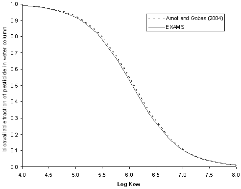
(Arnot and Gobas 2004)Parameter Symbol Definition Value Units XPOC concentration of particulate organic carbon in water user defined kg/L XDOC concentration of dissolved organic carbon in water user defined kg/L KOW octanol water partition coefficient user defined none Φ fraction of the overlying water concentration of the pesticide that is freely dissolved and can be absorbed via membrane diffusion calculated none αPOC Proportionality constant to describe the similarity of phase partitioning of POC in relation to octanol 0.35 none αDOC Proportionality constant to describe the similarity of phase partitioning of DOC in relation to octanol 0.08 none The Arnot and Gobas (2004) approach for calculating the fraction of bioavailable pesticide in the water column (Equation A2) is different from the approach used in EPA's Exposure Analysis Modeling System (EXAMS) (Equation A3, Table A3). The major difference is that the approach employed by EXAMS accounts for decreases in bioavailable pesticide in the water column due to sorption to biota. The values for αDOC for the two approaches are also slightly different. Despite these different approaches, for chemicals with Log KOW values 4-8, the fractions of bioavailable pesticide in the water column estimated by the two approaches differ by < 0.02 (Figure A1). Therefore, utilizing water column EECs generated by EXAMS is still consistent with the results that are generated using the approach described by Arnot and Gobas (2004).
Equation A3
F = 1 / [1 + (XPOC * αPOC * KOW) + (XDOC * αDOC * KOW) + (Xbiota * 0.436 * KOW0.907)]
Table A3
Equation A3: Derivation of Available Pesticide Fraction in Water (F) by EXAMS and Its Associated ParametersParameter Symbol Definition Value Units F fraction of the overlying water concentration of the pesticide that is freely dissolved and can be absorbed via membrane diffusion calculated none KOW octanol water partition coefficient user defined none OCSS percent organic carbon in suspended sediment user defined % XSS concentration of suspended sediments in water column user defined kg/m3 XPOC concentration of particulate organic carbon in water XSS*OCSS kg/m3 XDOC concentration of dissolved organic carbon in water user defined kg/m3 Xbiota concentration of biota in water user defined kg/m3 αPOC Proportionality constant to describe the similarity of phase partitioning of POC in relation to octanol 0.35 none αDOC Proportionality constant to describe the similarity of phase partitioning of DOC in relation to octanol 0.074 none  Figure A1
Fraction of bioavailable pesticide in water column estimated using approaches of Arnot and Gobas (2004) and EXAMS. Values for OCSS, XSS, XDOC and Xbiota are consistent with OPP standard pond scenario used in EXAMS. -
A.2 Calculation of Chemical Concentration in Sediment
Since it is possible for aquatic organisms to be exposed to chemicals through consumption of contaminated sediment, it is necessary to estimate the concentration of the chemical of concern in the sediment. This is accomplished using Equation A4 (Table A4), which uses the concentration of the chemical in the pore water, the chemical KOC, and the organic carbon content of the sediment. This approach is consistent with EXAMS for calculating the fraction of pesticide sorbed to sediment in the benthic column.
Equation A4
- CS = CSOC * OC
- where: CSOC = CWDP * KOC
Table A4
Equation A4: Derivation of Pesticide Concentration in the Solid Portion of the Sediment (CS)
(Arnot and Gobas 2004)Parameter Symbol Definition Value Units CS concentration of the chemical in sediment (dry weight of sediment) calculated g/(kg (dry) sediment) CSOC normalized (for OC content) pesticide concentration in sediment calculated g/(kg OC) CWDP freely dissolved pesticide concentration in pore water input parameter
(from PRZM/EXAMS)g/L KOC organic carbon partition coefficient user defined L/kg OC OC percent organic carbon in sediment user defined % -
A.3 Calculation of Respiration Uptake (k1) and Elimination (k2) Rate Constants
The respiratory uptake constant (k1) is calculated differently for phytoplankton (Equation A5.1) and for animals (Equation A5.2). For phytoplankton, k1 is dependent upon the KOW of the chemical as well as 2 constants (A and B) that describe chemical uptake resistance through the aqueous and organic phases (respectively) of the plant. If A and B are kept constant at 6x10⁻⁵ and 5.5, respectively as recommended by Arnot and Gobas (2004), k1 for phytoplankton increases with increasing KOW, ranging by a factor of 10 from Log KOW 4-8 (Figure A2).
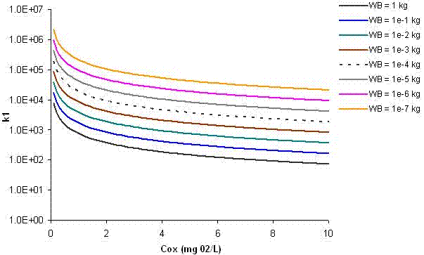
For animals, k1 is dependent upon the chemical uptake efficiency of the gills, the ventilation rate, and the body weight of the organism. The uptake efficiency of the gills is determined by the KOW of the chemical, while the ventilation rate of the organism is determined by an allometric equation that is influenced by the body weight of that organism and the concentration of oxygen in the water column (COX) (Table A5). When COX and organism body weight are kept constant, Log KOW has little effect on the k1 for animals (0.8% change from Log KOW 4-8). When Log KOW and body weight are kept constant, COX strongly affects k1. The value of k1 decreases by 50%, as the COX value increases from 5 to 10 mg/L (Figure A3). The value of k1 is also strongly influenced by the body weight of the organism, with decreasing k1 observed with increasing body weight. As the body weight of the organism increases from 1x10⁻⁷ to 10 kg (a relevant range for aquatic organisms, see Appendix C), the k1 value spans 3 orders of magnitude (Figure A3).
Equation A5.1
For phytoplankton: k1 = 1 / (A + B/KOW)
Equation A5.2
- For animals: k1 = (EW * GV) / WB
- where: EW = [1.85 + 155 / KOW]-1
- GV = 1400 * (WB0.65 / COX)
Table A5
Equations 5.1 and 5.2: Associated with the Derivation of Pesticide Clearance through the Respiratory (gill) System (k1) and Associated Parameters
(Arnot and Gobas 2004)Parameter Symbol Definition Value Units A constant related to the resistance to pesticide uptake through the aqueous phase of plant 6.0 x 10⁻⁵ (default) days B constant related to the resistance to pesticide uptake through the organic phase of plant 5.5 (default) days Cox concentration of dissolved oxygen User input (mg O2)/L EW pesticide uptake efficiency by gills (fraction) calculated none GV ventilation rate of fish, invertebrates, zooplankton calculated L/d k1 pesticide uptake rate constant through respiratory area
(i.e., gills, skin)calculated L/kg*d KOW octanol water partition coefficient user defined none WB wet weight of the organism user defined kg 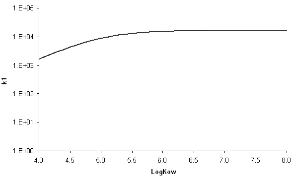 Figure A2
Relationship between Kow and k1 for phytoplankton. Figure A3
Relationship between COX, WB and k1 for aquatic animals.The elimination rate constant for the respiratory system (k2) is related to the respiratory uptake constants (k1). This is because both constants are influenced by the same processes related to respiration. The value of k2 is also influenced by the partitioning of the chemical between the organisms and the water. The organism-water partition coefficient (KBW) is determined by the body composition of the organism (i.e., lipid, NLOM, and water) and the KOW of the chemical. It is assumed that the partitioning of the chemical between lipid and water is directly related to the octanol-water partition coefficient. It is also assumed that the chemical partitioning between NLOM and water can be related to the octanol-water partition coefficient using a proportionality constant (β) (Equation A6, Table A6).
Equation A6
- k2 = k1 / kBW
- where: KBW = VLB * KOW + VNB * β * KOW + VWB
Table A6
Equation A6: Involved in the Derivation of the Respiratory Elimination Rate Constant (k2) and Associated Parameters
(Arnot and Gobas 2004)Parameter Symbol Definition Value Units k1 pesticide uptake rate constant for chemical uptake through respiratory area
(i.e., gills, skin, membrane permeation)calculated (Equation 5) L/kg*d k2 rate constant for elimination of the pesticide through the respiratory area
(i.e., gills, skin, membrane permeation)calculated d-1 KBW organism-water partition coefficient (based on wet weight) calculated none KOW octanol water partition coefficient user defined none VLB lipid fraction of organism user defined (kg lipid)/(kg organism wet weight) VNB - NLOM (Non Lipid Organic Matter) fraction of animals
- NLOC (Non Lipid Organic Carbon) of plants
user defined kg NLOM/(kg organism wet weight) VWB water content of the organism user defined kg water/(kg organism wet weight) β proportionality constant expressing the sorption capacity of NLOM or NLOC to that of octanol - Phytoplankton: 0.35
- Animals:0.035
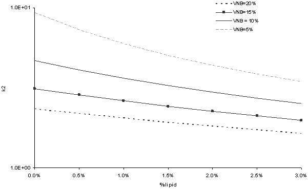
none Elimination rate constants for phytoplankton (k2) are calculated using seven parameters, including: KOW, VLB, VNB, VWB, A, B, and β (defined above in Table A6). The parameters A, B and β are all constants. If the other parameters are considered in terms of ranges applicable to KABAM, KOW has the greatest influence on the determination of k2 for phytoplankton. When Log KOW values are changed from 4 to 8, the k2 value decreases by three orders of magnitude (Figure A4). The lipid fraction of the organism (VLB) and the non-lipid organic carbon fraction (VNB) influence k2, with decreases in k2 observed as VLB and VNB increase. These two parameters are related. As VLB decreases, an increase in VNB has a greater effect on k2. Likewise, as VNB decreases, an increase in VLB has a greater effect on k2 (Figure A4). When the lipid fraction of organism (VLB) is increased from 0.5 to 3%, the elimination rate constant through respiration, i.e., k2, decreases by > 30% (Figure A5). A change in VNB from 5% to 20% results in a decrease in the value of k2 that is > 50% (Figure A5). The water content (VWB) of an organism has a negligible (< 0.5%) effect on k2.
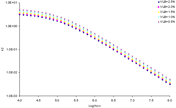 Figure A4
Influence of Log KOW on k2 (for phytoplankton) at different % lipid (VLB ).
(with VNB = 8%) Figure A5
Influence of % lipid (VLB) on k2 (for phytoplankton) at different % NLOM (VNB) at Log Kow 4.
Note that for all Log Kow values from 4-8, the curves follow a similar trend for different VLB and VNB, but differ in magnitude of k2.To determine elimination constant from respiration (k2) for animals, seven input parameters are required: KOW, WB, VLB, VNB, VWB, COX, and β (all of which are defined in Table A6). The parameter β is a constant representing the proportionality of the sorption of a chemical to NLOM to the KOW of that chemical. If the other parameters are considered in terms of ranges applicable to KABAM, the octanol-water partition coefficient (KOW) and the water content of the organism (VWB) have the greatest influence on the determination of k2. When Log KOW values are changed from 4 to 8, the k2 value decreases by 4 orders of magnitude (Figures A6 and A7). Body weight also influences k2, with k2 values decreasing by 2 orders of magnitude as the body weight is increased from 1x10⁻⁷ to 1 kg (this is a range considered relevant to aquatic animals, see Appendix C for more information) (Figure A6). The lipid fraction of the organism (VLB) and the non-lipid organic matter fraction (VNB) influence k2, with decreases in k2 observed as these two values increase. When VLB is increased from 1 to 5%, k2 decreases by 84% (Figure A7). When VNB is increased from 15 to 40%, a 14% decrease in k2 is observed. The water content (VWB) of an organism has a negligible (< 0.5%) effect on k2. Increasing the concentration of the dissolved oxygen (COX) value from 5 to 10 mg/L results in a decrease of 50% in the value of k2.
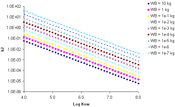 Figure A6
Influence of Log KOW on k2 (for animals) at different body weights (WB).
(with VLB = 5%, VNB = 20%, VWB = 75% and COX = 10mg/L)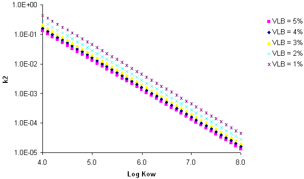 Figure A7
Influence of Log KOW on k2 (for animals) at different % lipid composition (VLB).
(with WB = 1 kg, VNB = 20%, VWB = 75% and COX = 10 mg/L) -
A.4 Calculation of Growth Rate Constant
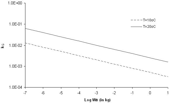
Equations A7.1 and A7.2 provide an approximation of growth of aquatic organisms based on weight and temperature (Table A7). Comparing the results of the two equations indicates that higher temperatures result in higher growth rate constant (kG) values (Figure A8). With both equations, as body weight increases, kG decreases. There is some uncertainty associated with these equations, since growth rate can be influenced by additional factors, including species and prey availability. For KABAM, it is assumed that if the water temperature (T) < 17.5 °C (midpoint between 10 and 25 °C), equation A.7.1 is used and if T ≥ 17.5 ° C, equation A.7.2 is used.
Equation A7.1
kG = 0.0005 * WB-0.2 (T ≈ 10 °C)
Equation A7.2
kG = 0.00251 * WB-0.2 (T ≈ 25 °C)
Table A7
Equations A7.1 and A7.2: Involving the Derivation of the Growth Rate Constant (kG) and Associated Parameters
(Arnot and Gobas 2004).Parameter Symbol Definition Value Units kG organism growth rate constant calculated d-1 T temperature user defined °C WB wet weight of the organism user defined kg 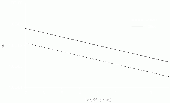 Figure A8
Relationship between body weight (WB) and kG at 2 different temperatures. -
A.5 Calculation of Dietary Uptake (kD) Rate Constant
In determining uptake and elimination rate constants related to dietary sources of chemicals (kD and kE, respectively), it is assumed that aquatic organisms are represented by a 2-phase model that includes the gastrointestinal tract (GIT) of the organisms and the organism itself. Since phytoplankton do not consume other organisms, a dietary uptake constant (kD) is not a relevant rate constant, and the elimination rate constant due to fecal elimination (kE) is considered insignificant in plants. Therefore, kD and kE are only calculated for animals.
The dietary uptake constant for a chemical in animals is influenced by the weight of the organism, the feeding rate of the organism (GD), and the dietary pesticide transfer efficiency (ED). The feeding rate is different for filter feeders compared to other aquatic organisms. Empirical dietary pesticide transfer efficiency (ED) values vary from 0-100%. Variability in ED has been attributed to various factors, including sorption coefficients of chemicals, composition of diet, and digestibility of diet. Based on several different observations, it is assumed by Arnot and Gobas (2004) that this value can be related to KOW (Equation A8, Table A8).
Equation A8
- kD = ED * (GD / WB)
- where: ED = (3.0x10⁻⁷ * KOW + 2.0)-1
- For animals (except filter feeders): GD = 0.022 * WB0.85 * exp(0.06 * T)
- For filter feeders: GD = GV * CSS * σ
- GV = 1400 * (WB0.65 / COX)
Table A8
Equation A8: Involving the Derivation of the Pesticide Clearance Rate Constant through Diet (kD) and Associated Parameters
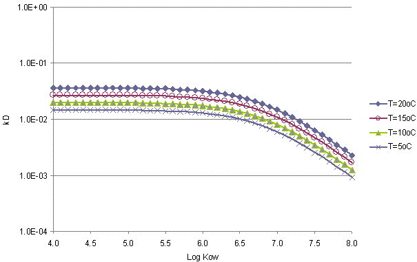
(Arnot and Gobas 2004)Parameter Symbol Definition Value Units Cox concentration of dissolved oxygen user defined (mg O2)/L CSS concentration of suspended solids user defined kg/L ED dietary pesticide transfer efficiency calculated % GD feeding rate of organism calculated kg/d GV ventilation rate of gills calculated L/d kD pesticide uptake rate constant for uptake through ingestion of food calculated kg food/(kg org*day) KOW octanol water partition coefficient user defined none T temperature user defined °C WB wet weight of the organism user defined kg σ efficiency of scavenging of particles absorbed from water 100 % For aquatic organisms (non-filter feeders), the dietary uptake constant (kD) is derived using 3 input parameters: octanol-water partition coefficient (KOW), the weight of the organism (WB), and temperature (T). For chemicals with Log KOW ranging 4-5.5, changes in Log KOW cause little (< 4%) effects to the value of kD; however, for chemicals with Log KOW < 5.5, increases in Log KOW can result in decreases in this value up to an order of magnitude (Figure A9). Increases in WB from 1x10⁻⁷ to 1 kg result in an order of magnitude decrease in kD (Figure A9). Temperature also affects kD, with an observed increase in kD of 65% when the temperature is increased from 2.5 to 20 °C (Figure A10).
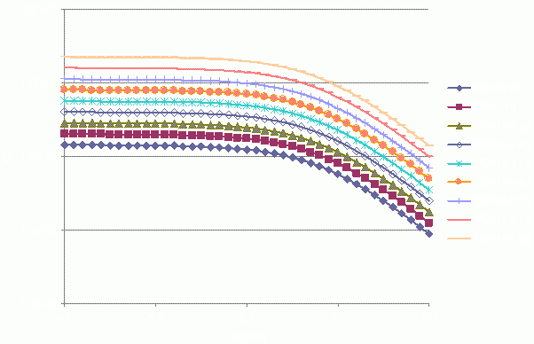 Figure A9
Relationship between Log KOW and kD (for non-filter feeders) at different body weights (WB).
(T=10 °C)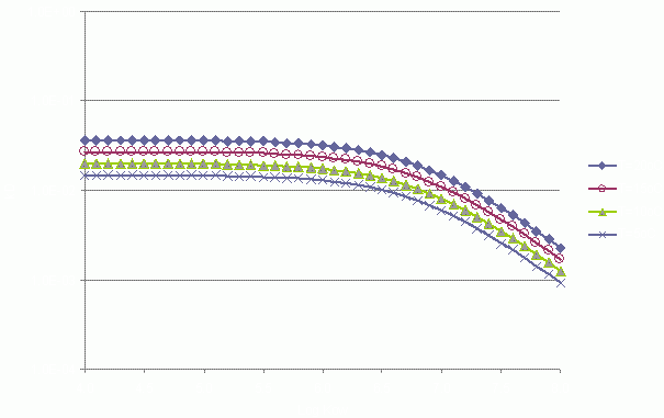 Figure A10
Relationship between Log KOW and kD (for non-filter feeders) at different water temperatures.
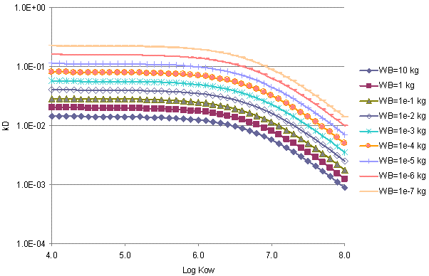
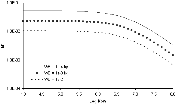
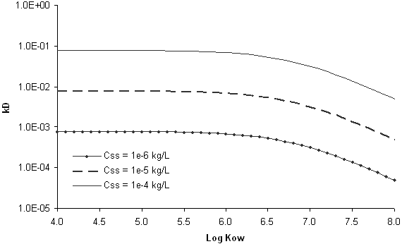
(WB=1 kg)For filter feeders, the dietary uptake constant (kD) is derived using five input parameters: KOW, WB, COX, CSS and σ (all of which are defined in Table A.8). For chemicals with Log KOW values ranging 4-5.5, changes in Log KOW cause little (< 5%) effects to the value of kD; however, as the Log KOW increases from 6 to 8, the kD for filter feeders decreases by an order of magnitude (Figure A11). Available National Water Quality Assessment (NAWQA) data for streams indicate that suspended sediment concentrations range 1-281 mg/L (USGS 2008b). If the concentration of suspended sediments (CSS) is increased from 1x10⁻⁶ to 1x10⁻⁴ kg/L, kD for filter feeders increases by 2 orders of magnitude (Figure A12). Increases in WB from 1x10⁻⁴ to 1x10⁻² kg (which is a reasonable range of weights for filter feeders; see Appendix C) result in an 80% decrease in kD (Figure A11). Increases in oxygen concentration (COX) from 2 to 8 mg/L results in a decrease in kD of 80% for filter feeders. Changes in the scavenging efficiency (σ) of filter feeders result in proportional changes to the kD value. For example, a 25% decrease in σ results in a 25% decrease in kD.
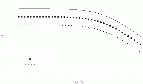 Figure A11
Relationship between Log KOW and filter feeder kD with different WB values.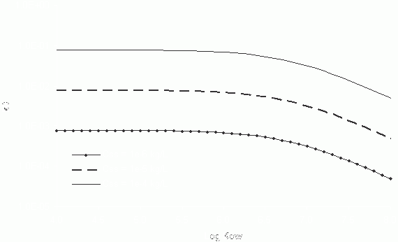 Figure A12
Relationship between Log KOW and filter feeder kD with different Css values. -
A.6 Calculation of Dietary Elimination (kE) Rate Constant
The rate constant for elimination of the pesticide through excretion of contaminated feces (kE) is calculated using the fecal egestion rate (GF), the dietary pesticide transfer efficiency (ED), the partition coefficient of the pesticide between the gastro-intestinal tract and the organism (KGB), and the body weight of the organism (WB) (Equation A9, Table A9). For filter-feeding and non-filter feeding aquatic animals, kE is calculated in a similar manner, with the exception of the method of calculating the feeding rate of an organism (GD). An order of magnitude increase in either GF, ED, or KGB results in an order of magnitude increase in fecal egestion rate constant (kE). An order of magnitude increase in WB results in an order of magnitude decrease in kE. Effects of changes in individual input parameters used to derive GF, ED, and KGB are explored below.
Equation A9
- kE = GF * ED * (KGB / WB)
- where: ED = (3.0x10⁻⁷ * KOW + 2.0)-1
- KGB = (VLG * KOW + VNG * β * KOW + VWG) / (VLB * KOW + VNB * β * KOW + VWB)
- VLG = [(1-εL) * VLD] / [(1-εL) * VLD + (1-εN) * VND + (1-εW) * VWD]
- VNG = [(1-εN) * VND] / [(1-εL) * VLD + (1-εN) * VND + (1-εW) * VWD]
- VWG = [(1-εW) * VWD] / [(1-εL) * VLD + (1-εN) * VND + (1-εW) * VWD]
- GF = [(1-εL) * VLD + (1-εN) * VND + (1-εW) * VWD] * GD
- For animals (except filter feeders): GD = 0.022 * WB0.85 * exp(0.06 * T)
- For filter feeders: GD = GV * CSS * σ
- GV = 1400 * (WB0.65 / COX)
Table A9
Equation A9: Involving the Derivation of the Fecal Elimination Rate Constant (kE) and Associated Parameters
(Arnot and Gobas 2004)Parameter Symbol Definition Value Units Cox concentration of dissolved oxygen calculated (mg O2)/L CSS concentration of suspended solids user defined kg/L ED dietary pesticide transfer efficiency calculated % GD feeding rate of organism calculated kg/d GF egestion rate of fecal matter calculated (kg feces)/(kg organism)*d GV ventilation rate of gills calculated L/d kE rate constant for elimination of the pesticide through excretion of contaminated feces - for animals: calculated
- for plants: 0
d-1 KGB partition coefficient of the pesticide between the gastro-intestinal tract and the organism calculated none KOW octanol water partition coefficient user defined none T temperature user defined °C VLB lipid fraction of organism user defined (kg lipid)/(kg organism wet weight) VLD overall lipid content of diet user defined kg/kg VLG lipid content in the gut calculated (kg lipid)/(kg digesta wet weight) VNB - NLOM (Non Lipid Organic Matter) fraction of animals
- NLOC (Non Lipid Organic Carbon) of plants
user defined kg NLOM/(kg organism wet weight) VND overall NLOM content of diet user defined kg/kg VNG NLOM content in the gut calculated (kg NLOM)/(kg digesta wet weight) VWB water content of the organism user defined kg water/(kg organism wet weight) VWD overall water content of diet user defined kg/kg VWG water content in the gut calculated (kg water)/(kg digesta wet weight) WB wet weight of the organism user defined kg β proportionality constant expressing the sorption capacity of NLOM to that of octanol 0.035 for animals none εL dietary assimilation rate of lipids - fish: 92%
- aquatic inverts: 75%
- zooplankton: 72%
% εN dietary assimilation rate of NLOM - fish: 60%
- aquatic inverts: 75%
- zooplankton: 72%
% εW dietary assimilation rate of water freshwater organisms: 25% % σ efficiency of scavenging of particles absorbed from water 100 % -
A.6.1 Parameters Affecting GF
The fecal egestion rate GF is calculated using the feeding rate of the organism (GD; kg/day), the dietary assimilation rates for lipids, NLOM, and water (εL, εN and εW, respectively) as well as the contents of the diet (VLD, VND, and VWD).
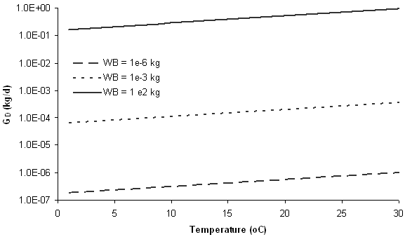
For non-filter feeders, the feeding rate (GD) is calculated using body weight and temperature. Generally, as body weight and temperature increase, so does the feeding rate of the aquatic animal (Figure A.13). An order of magnitude increase in body weight leads to an order of magnitude increase in the feeding rate of the organism. An order of magnitude increase in temperature leads to a 40% increase in the feeding rate of non-filter feeders.
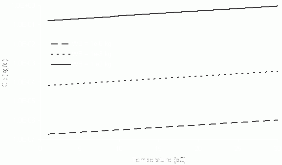 Figure A13
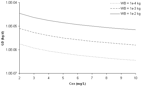
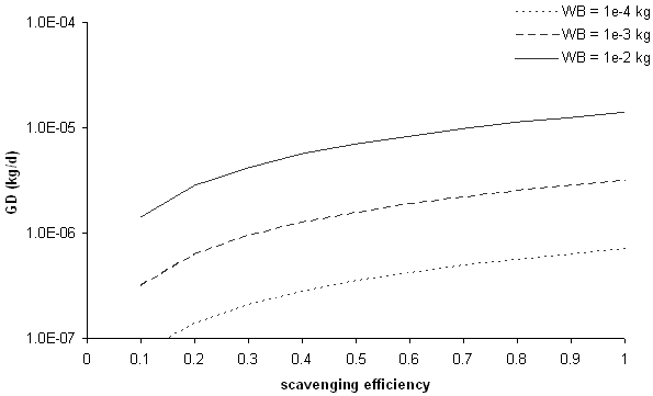
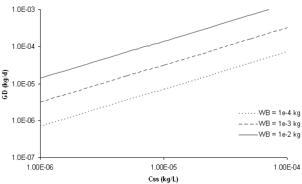
Relationship between temperature and GD (non-filter feeders) with different WB values.For filter feeders, the feeding rate (GD) is calculated using four parameters: the concentration of dissolved oxygen in the water (COX), body weight (WB), the concentration of suspended solids (CSS), and the scavenging efficiency of particles absorbed from water (σ). As with non-filter feeders, increases in body weight of filter feeders leads to increases in GD (Figures A14-A16). An order of magnitude increase in body weight leads to an 80% increase in feeding rate (GD). An increase in dissolved oxygen in the water (COX) from 2 to 10 mg/L results in a decrease in GD of 80% (Figure A14). Decreases in scavenging efficiency lead to proportional decreases in GD, with every 10% decrease in scavenging efficiency (σ), leading to a 10% decrease in GD (Figure A15). An order of magnitude increase in the concentration of suspended solids (CSS) leads to an order of magnitude increase in GD (Figure A16).
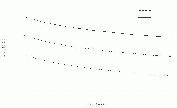 Figure A14
Relationship between Cox and GD (filter feeders) with different WB values.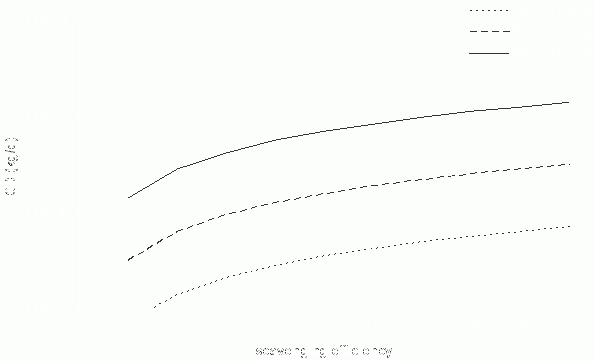 Figure A15
Relationship between scavenging efficiency and GD (filter feeders) with different WB values.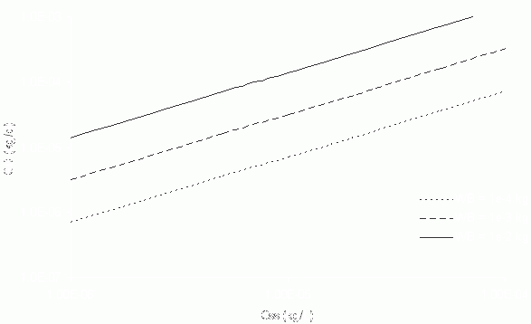 Figure A16
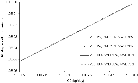
Relationship between concentration of suspended solids (Css) and GD (filter feeders) with different WB values.The fecal egestion rate (GF) is calculated using the following parameters: εL, εN, εW, VLD , VND, VWD as well as GD, which is discussed above. When the default dietary assimilation rates for lipids, NLOM, and water (εL, εN, and εW, respectively) are used, changes in lipid, NLOM and water composition of the diet (VLD, VND and VWD, respectively) have little effect on GF, when compared to effects of GD on GF (Figure A.17). This indicates that as the feeding rate of an animal (GD) increases so does its fecal egestion rate (GF), while the composition of the animal's diet has little effect on the fecal egestion rate.
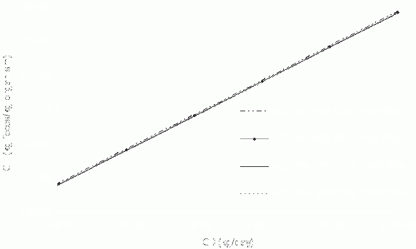 Figure A17
Relationship between GD and GF with different lipid, NLOM, and water compositions in the diet
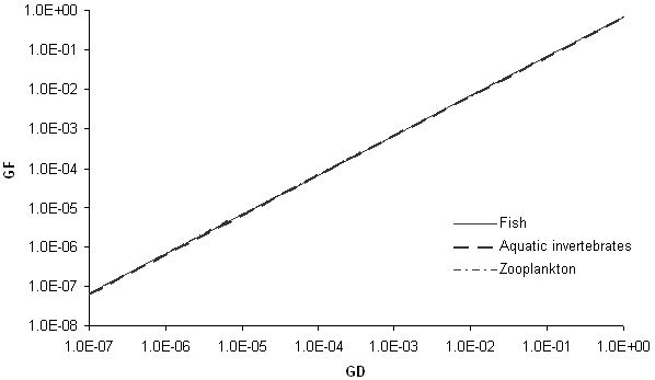
(VLD, VND, and VWD, respectively). Dietary assimilation rates for lipids, NLOM, and water are set to default values used to represent fish (see Table A9).When setting the lipid, NLOM, and water composition (VLD, VND and VWD, respectively) of diet equal for fish, aquatic invertebrates, and zooplankton, the differences in dietary assimilation rates for lipids, NLOM, and water (εL, εN, and εW, respectively) of these three groups of animals have little effect on the fecal egestion rate (GF), when compared to effects of the feeding rate (GD) on GF (Figure A.18). As with the composition of the diet, changes in GD result in greater effects on GF when compared to changes in the assimilation efficiencies of lipid, NLOM, and water.
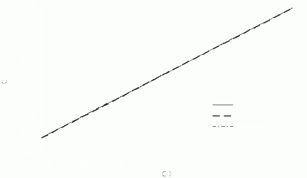 Figure A18
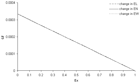
Relationship between GD and GF with dietary assimilation rates for lipids, NLOM, and water set to default values for fish, aquatic invertebrates, and zooplankton (see Table A9). Lipid, NLOM, and water compositions in the diet (VLD, VND, and VWD, respectively) are set to 1, 20, and 79%, respectively.When VLD, VND, VWD are equal (i.e., 33.33%) and when GD is set to a constant number, variations of εL, εN, and εW result in equivalent effects to GF, with GF decreasing as assimilation efficiency increases (i.e., the organism eliminates less as its digestion [assimilation efficiency] becomes more efficient). If assimilation efficiency is set to 1 for lipid, NLOM, and water, the fecal elimination rate of the organism is 0 kg feces/kg org (Figure A.19).
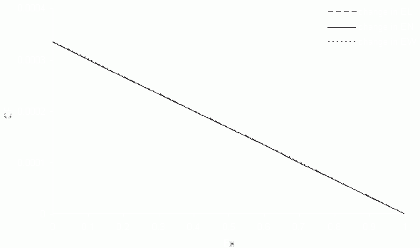 Figure A19
Relationship between dietary assimilation efficiencies (εL, εN, and εW) and GF (VLD=VND=VWD=33.33%; GD = 1.0x10⁻³ kg/day).
Each dietary efficiency rate was altered independent of the others, with the others set to 1.In summary, changes in the feeding rate of the organism (GD) have the greatest effect on the fecal egestion rate of the organism (GF). GD is calculated for non-filter feeders using body weight and temperature. GD is calculated for filter feeders, using the concentration of dissolved oxygen in the water (COX), body weight (WB), the concentration of suspended solids (CSS), and the efficiency of scavenging of particles absorbed from water (σ). Changes in these parameter values would be expected to have the greatest influence on GF, which would result in influences on rate constant for pesticide elimination through excretion (kE). Changes in the composition of the diet and the dietary assimilation rates are expected to have less of an influence on GF when compared to GD and the parameters used to derive GD.
-
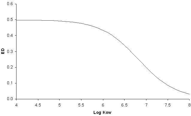
A.6.2 Parameters Affecting ED
The efficiency of dietary pesticide transfer (ED) is based only upon the KOW of the pesticide. As KOW increases, ED decreases. For chemicals with Log KOW 4-8, the efficiency of dietary pesticide transfer is 50-3% (Figure A.20).
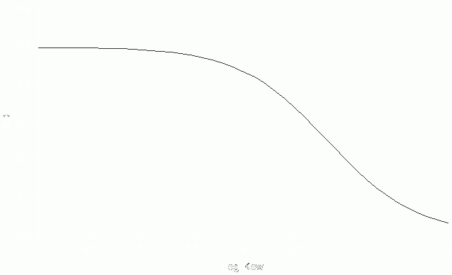 Figure A20
Dietary transfer efficiency (ED) vs. Log Kow -
A.6.3 Parameters Affecting KGB
The equations used to calculate the contents of the gut (i.e., VLG, VNG, and VWG) listed in Table A.9 can be simplified as follows, using the equation for GF:
VLG = [(1 - εL) * VLD * GD] / GF
VNG = [(1 - εN) * VND * GD] / GF
VWG = [(1 - εW) * VWD * GD] / GF
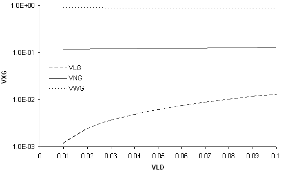
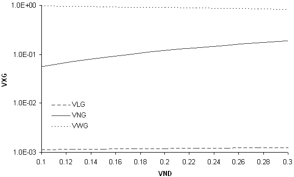
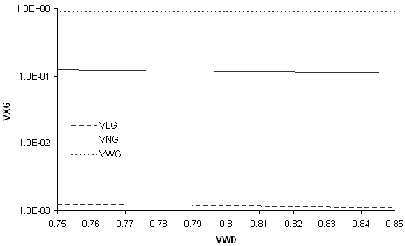
Using these simplified equations, changes in the feeding rate of the organism (GD), the fecal egestion rate (GF), diet composition, and dietary assimilation of lipid, NLOM, and water can be explored to understand effects on these parameters on estimations of the lipid composition of the gut. If εL, εN, and εW are all equal and VLD, VND, and VWD are all equal, VLG, VNG, and VWG are equal. Changes in feeding rate (GD) and fecal egestion rate (GF) do not affect VLG, VNG or VWG (Figure A.21). As would be expected, changes in VLD result in effects to VLG, with an order of magnitude increase in VLD, resulting in an order of magnitude increase in VLG (Figure A.22). Also, changes in VND result in effects to VNG, with an increase in VND from 10 to 20%, resulting in a 50% increase in VNG (Figure A.23). An order of magnitude increase in VWD (keeping VLD and VND constant) results in slight (approximately 10%) decreases in VLG and VNG and slight (2%) increases in VWG (Figure A.24). A decrease in εL from 0.9 to 0.1, results in an order of magnitude increase in the lipid content of the gut (VLG) (Figure A.25), but only slight (< 2%) changes to the NLOM and water contents of the gut (VNG and VWG, respectively). A decrease in εN from 0.9 to 0.1 results in an order of magnitude increase in the NLOM content of the gut (VNG) (Figure A.26), as well as decreases in the gut composition attributed to lipid and water. A decrease in εW from 0.9 to 0.1 results in a 50% increase in the water content of the gut (VWG), as well as an 80% decrease in the gut composition attributed to lipid and NLOM (Figure A.27). For invertebrates, dietary assimilation efficiencies vary significantly, leading to uncertainty in assigning one value to this parameter. Since hydrophobic chemicals are not likely to be stored in the water of organism tissues, it is assumed that this route is not significant to bioaccumulation.
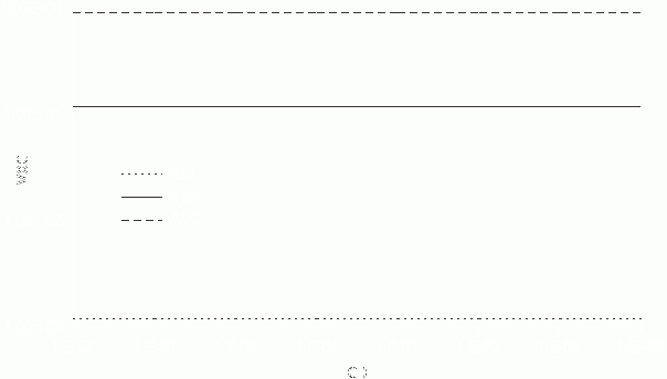 Figure A21
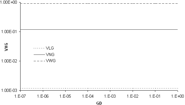
Relationship between gut contents (VLG, VNG, and VWG) and GD.
εL, εN, and εW are set to defaults for fish (Table A9).
VLD = 1%, VND = 20%, and VWD = 79%.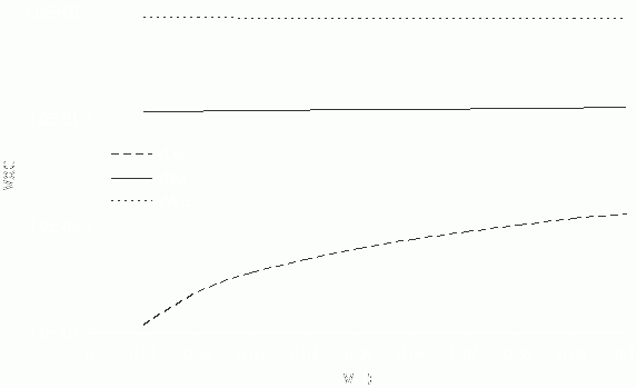 Figure A22
Relationship between gut contents (VLG, VNG, and VWG) and VLD.
εL, εN, and εW are set to defaults for fish (Table A9).
VND = 20%, VWD = 1-VND-VLD.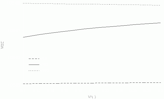 Figure A23
Relationship between gut contents (VLG, VNG, and VWG) and VND.
εL, εN, and εW are set to defaults for fish (Table A9).
VLD = 1%, VWD = 1-VND-VLD.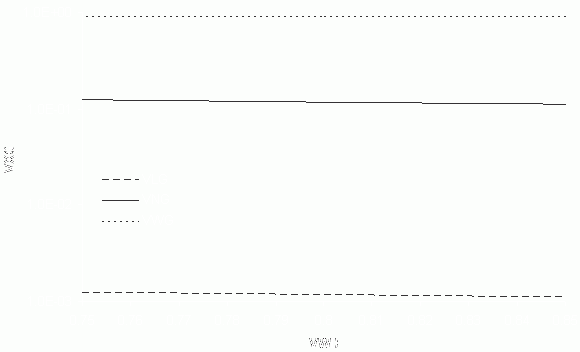 Figure A24
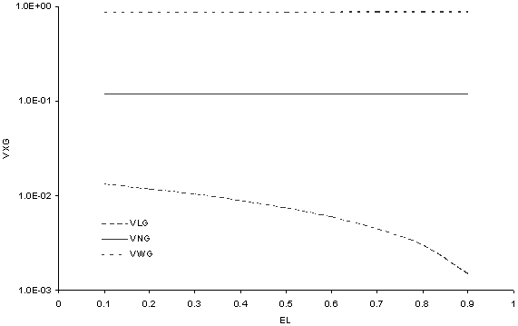
Relationship between gut contents (VLG, VNG, and VWG) and VWD.
εL, εN, and εW are set to defaults for fish (Table A9).
VLD = 1%, VND = 20%.
Note that VLD+VND+VWD does not equal 100%, except when VWD = 0.79.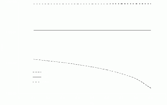 Figure A25
Relationship between gut contents (VLG, VNG, and VWG) and εL.
εN, and εW are set to defaults for fish (Table A9).
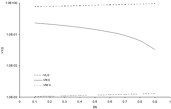
VLD = 1%, VND = 20%, VWD = 79%.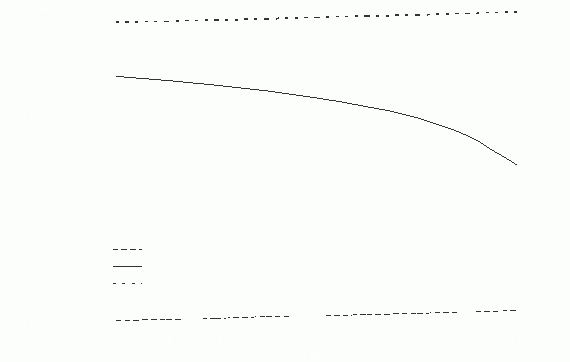 Figure A26
Relationship between gut contents (VLG, VNG, and VWG) and εN.
εL, and εW are set to defaults for fish (Table A9).
VLD = 1%, VND = 20%, VWD = 79%.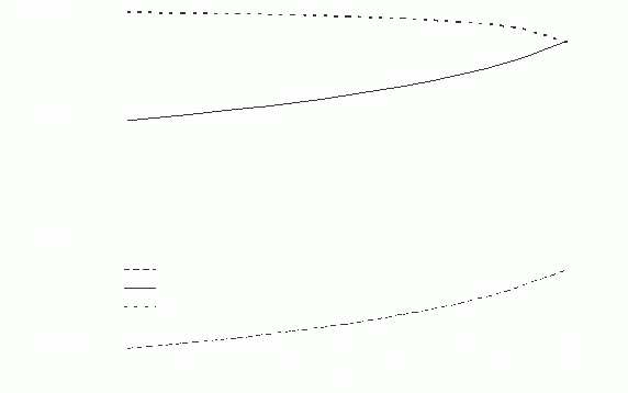 Figure A27
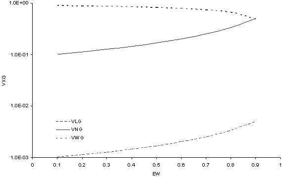
Relationship between gut contents (VLG, VNG, and VWG) and εW.
εL, and εN are set to defaults for fish (Table A9).
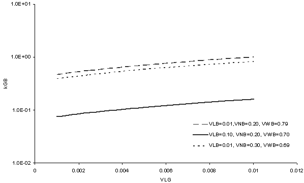
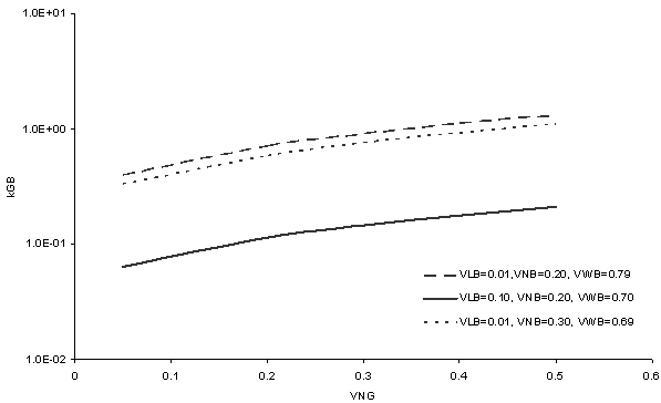
VLD = 1%, VND = 20%, VWD = 79%.The partitioning of a chemical between the gastrointestinal tract (GIT) and the organism is described by KGB. This partition coefficient is determined using the contents of the gut (VLG, VNG, and VWG), the contents of the organism's body (VLB, VNB and VWB) as well as the octanol water partition coefficient (KOW) (Table A.9). An order of magnitude increase in the lipid content of the body (VLB) results in an order of magnitude decrease in KGB (Figures A.28 and A.29). An order of magnitude increase in the NLOM content of the body (VNB) results in a decrease in KGB of approximately 20%. An order of magnitude increase in the lipid content of the gut (VLG) results in a 50% increase in KGB (Figure A.28). An order of magnitude increase in the NLOM content of the gut (VNG), results in an increase in KGB of 70% (Figure A.29). Changes in the Log KOW of a chemical from 4 to 8 do not alter KGB.
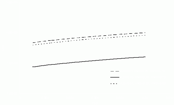 Figure A28
Relationship between lipid content of the gut (VLG) and KGB,
with different body compositions (VLB, VNB, and VWB).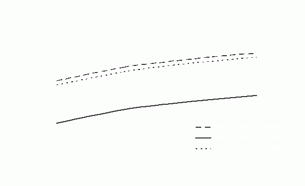 Figure A29
Relationship between NLOM content of the gut (VNG) and KGB,
with different body compositions (VLB, VNB, and VWB).
-
A.7 Overall Sensitivity of Body Concentration of Chemical (CB) to Individual Input Parameters
-
A.7.1. First Sensitivity Analysis
In order to understand the influence of input parameters on model predictions of pesticide concentrations in tissue of aquatic organisms (CB), a sensitivity analysis was conducted. Parameters were assigned uniform distributions and assumptions of ranges based on data in the scientific literature. The range for each parameter is defined in Table A10. Diets of each trophic level were varied according to the definitions in Table A11. Uniform distributions were used to allow unbiased selection of values from set ranges. Once parameter assumptions were assigned, a Monte Carlo simulation was carried out using Crystal Ball 2000. In this simulation, 10,000 trials were conducted with randomly selected parameter values resulting in predicted pesticide concentrations in each of the seven trophic levels. The sensitivity of the model to specific parameters was defined by the contribution of each parameter to the variance of the estimation of pesticide concentrations in each of the trophic levels.
The results of this analysis indicate that of all the variables in the model, the Log KOW contributes the most to variability (< 75% of total) in estimates of CB for all animal trophic levels. For phytoplankton, the water column EEC, concentration of POC in the water column (XPOC) and Log KOW contribute the greatest variability in the predicted CB values (38, 28, and 22%, respectively).
-
A.7.2. Second Sensitivity Analysis
Based on the results of the first sensitivity analysis, a second analysis was conducted where the influence of individual parameters on variability in CB was examined, with fixed Log KOW values. In the second sensitivity analysis, the Log KOW was set to values of 4, 5, 6, 7, and 8 and a Monte Carlo simulation (10,000 trials) was run for each Log KOW value. Parameters were assigned uniform distributions and assumptions of ranges based on data in the scientific literature. The range for each parameter is defined in Table A10 (with the exception of Log KOW). Diets of each trophic level were varied according to the definitions in Table A11.
The contributions of individual parameters at Log KOW values of 4, 5, 6, 7 and 8 to the variability in the pesticide tissue concentration (CB) of the seven aquatic trophic levels of KABAM are provided in Tables A12-A18. The results of this sensitivity analysis indicate that parameters have different relative importance in estimating CB for the seven trophic levels (e.g., the water column EEC contributes the most variability to the phytoplankton CB, while the pore water EEC and fraction of respiratory ventilation that involves pore-water of sediment (mP) value contribute the most variance to the zooplankton CB). In addition, these tables indicate that the relative importance of individual parameters to estimates of CB change with Log KOW. It should be noted that several parameters in the Arnot and Gobas (2004) model are linked (e.g., mP and mO, diet composition, VLB, VNB, and VWB). Therefore, sensitivity of CB predictions to one parameter implies sensitivity of the predictions to the linked parameters.
This sensitivity analysis also indicates that some parameters that are fixed in KABAM, including the constant related to the resistance to pesticide uptake through the aqueous phase of plant (A), proportionality constant expressing the sorption capacity of NLOM to that of octanol (β), and mP (set to either 0 or 0.05), can contribute > 10% of total variability in estimates of CB.
Table A10
Parameters and Associated Assumptions Used for First and Second Sensitivity Analysis of KABAMParameter Parameter Description Trophic Level Minimum of Range Maximum of Range Source/Comments A Constant related to the resistance to pesticide uptake through the aqueous phase of plant Phytoplankton 1x10⁻⁵ 1x10⁻⁴ In Arnot and Gobas 2004, this value is set to a constant of 6.0x10⁻⁵ days. This value was varied by an order of magnitude around the reported constant value to understand the influence of this parameter on estimates of bioaccumulation. The reasonable range of values for this parameter is unknown. B Constant related to the resistance to pesticide uptake through the organic phase of plant Phytoplankton 1 10 In Arnot and Gobas 2004, this value is set to a constant of 5.5 days. This value was varied by an order of magnitude around the reported constant value to understand the influence of this parameter on estimates of bioaccumulation. The reasonable range of values for this parameter is unknown. COX Concentration of dissolved oxygen (mg O2/L) All 4 12 Minimum is based on 60% of saturation of water with 6 mg/L as saturation (in 30 °C water). Maximum is based on solubility limit of oxygen in cold water (5 °C; see USGS 2008a). CSS Concentration of suspended solids (kg/L) All 2.0x10⁻⁶ 5.0x10⁻⁴ Based on 5th and 95th percentiles of approximately 38,000 measurements of suspended sediment concentrations in surface waters of the US provided by NAWQA (USGS 2008b). CWTO Total pesticide concentration in water column above the sediment All 0.1 100 Assumed to be reasonable range for EECs expected from PRZM/EXAMS modeling. CWTP Freely dissolved pesticide concentration in pore water of sediment All 0.1 100 Assumed to be reasonable range for EECs expected from PRZM/EXAMS modeling. Log Kow Log of octanol-water partition coefficient All 4 8 Assumption that bioaccumulation model can be used for chemicals with Log Kow 4-8. Koc Organic carbon partition coefficient All 3.5x10³ 3.5 x10⁷ Determined based on assumption that Koc can be estimated as 0.35*Kow. In sensitivity analysis, Koc is linked directly to KOW in order to avoid error in selection of inconsistent values for these parameters. mp Fraction of respiratory ventilation that involves pore-water of sediment Zooplankton 0 1 Based on full range of parameter values. Benthic Inv. 0 1 Based on full range of parameter values. Filter Feeders 0 1 Based on full range of parameter values. Small Fish 0 1 Based on full range of parameter values. Medium Fish 0 1 Based on full range of parameter values. Large Fish 0 1 Based on full range of parameter values. OC Percent organic carbon in sediment All 1% 10% In the OPP standard pond used in EXAMS, the default value for this parameter is 4%. This parameter value is varied by 1 order of magnitude around the OPP standard pond value. T Temperature (°C) All 1 30 Reasonable range of values for this parameter in the environment. VLB Lipid fraction of organism Phytoplankton 0.5 2.0 See Table C1 of Appendix C. Zooplankton 1.0 4.0 See Table C2 of Appendix C. Benthic Inv. 0.5 12 See Tables C4-C9 of Appendix C. Filter Feeders 0.4 4 See Tables C13-C15 of Appendix C. Fish 0.5 8 See Table C19 of Appendix C. VNB - NLOM (Non Lipid Organic Matter) fraction of animals
- NLOC (Non Lipid Organic Carbon) of plants
All - - Set to equal 1-VLB-VWB VWB Water content of the organism Phytoplankton 0.85 0.95 Assume 5% deviation from mean (i.e., 90%). Zooplankton 0.74 0.96 See Section C.2. of Appendix C. Benthic Inv. 0.69 0.83 See Table C3 of Appendix C. Filter Feeders 0.78 0.93 See Table C12 of Appendix C. Fish 0.71 0.80 See Table C18 of Appendix C. WB Wet weight (kg) of the organism Phytoplankton - - Not a necessary parameter for phytoplankton. Zooplankton 1x10⁻⁹ 1x10⁻⁷ See Section C.2. of Appendix C. Benthic Inv. 5x10⁻⁶ 2x10⁻³ See Table C11 of Appendix C. Filter Feeders 2x10⁻⁴ 1x10⁻² See Section C.5 of Appendix C. Small Fish 1x10⁻³ 5x10⁻² See Table C16 of Appendix C. Medium Fish 5x10⁻³ 0.6 See Table C17 of Appendix C. Large Fish 0.25 3.6 See Section C.5 of Appendix C. XPOC Concentration of particulate organic carbon in water (kg/L) All 2.0x10⁻⁶ 5.0x10⁻⁴ Based on 5th and 95th percentiles of approximately 38,000 measurements of suspended sediment concentrations in surface waters of the US provided by NAWQA (USGS 2008b). XDOC Concentration of dissolved organic carbon in water (kg/L) All 5.0x10⁻⁷ 5.0x10⁻⁵ In the OPP standard pond used in EXAMS, the default value for this parameter is 5.0x10⁻⁶. This parameter value is varied by 2 orders of magnitude around the OPP standard pond value. β Proportionality constant expressing the sorption capacity of NLOM or NLOC to that of octanol All 0 1 Designed to represent all values equal to or less than the partitioning of a chemical between octanol and water. εL Dietary assimilation rate of lipids Animals 0 1 Based on full range of parameter values. εN Dietary assimilation rate of NLOM Animals 0 1 Based on full range of parameter values. εW Dietary assimilation rate of water Animals 0 1 Based on full range of parameter values. σ Efficiency of scavenging of particles absorbed from water Filter Feeders 0 1 Based on full range of parameter values. Table A11
Dietary Assumptions of Aquatic Trophic Levels Used for Sensitivity Analysis of KABAMTrophic Level Organism in diet Minimum Value Maximum Value Comments Zooplankton Phytoplankton 100% 100% - Benthic Invertebrates Sediment 0 50% - Phytoplankton 0 50% - Zooplankton - - Set to 1- (% diet attributed to sediment + % diet attributed to phytoplankton) Filter Feeder Sediment 0 33% - Phytoplankton 0 33% - Zooplankton 0 33% - Benthic invertebrates - - Set to 1- (% diet attributed to sediment + % diet attributed to phytoplankton + % diet attributed to zooplankton) Small Fish Phytoplankton 0 50% - Zooplankton 0 50% - Benthic invertebrates - - Set to 1- (% diet attributed to phytoplankton + % diet attributed to zooplankton) Medium Fish Zooplankton 0 50% - Benthic invertebrates 0 50% - Small fish - - Set to 1- (% diet attributed to zooplankton + % diet attributed to benthic invertebrates) Large Fish Small fish 0 100% It is assumed that large fish consume only smaller fish Medium Fish - - Set to 1- (% diet attributed to small fish) Table A12
Second Sensitivity Analysis Results: Contribution to Variance of Specific Variables to CB Values of Phytoplankton at Different Log Kow ValuesVariable 4 5 6 7 8 A ≤ 0.1% ≤ 0.1% 0.7% 9.3% 18.2% VLB ≤ 0.1% ≤ 0.1% ≤ 0.1% 0.2% ≤ 0.1% VWB 5.9% 3.4% 2.3% 0.2% ≤ 0.1% Water Column EEC 59.6% 46.1% 44.9% 45.7% 43.0% XPOC 7.0% 30.9% 39.1% 41.7% 38.0% β 26.7% 18.6% 12.0% 2.1% ≤ 0.1% Total 99.2% 99.0% 99.0% 99.2% 99.2% Table A13
Second Sensitivity Analysis Results: Contribution to Variance of Specific Variables to CB Values of Zooplankton at Different Log Kow ValuesVariable 4 5 6 7 8 COX ≤ 0.1% ≤ 0.1% 0.2% 2.5% 4.3% mP 4.3% 23.0% 37.4% 39.5% 36.1% Pore Water EEC 27.6% 37.2% 40.8% 40.6% 37.4% T ≤ 0.1% ≤ 0.1% 1.3% 7.7% 19.6% VLB 1.2% 0.4% 0.6% 0.6% ≤ 0.1% VWB 20.8% 14.1% 8.8% 0.6% 0.8% Water Column EEC 11.2% 2.2% 0.3% ≤ 0.1% ≤ 0.1% WB ≤ 0.1% ≤ 0.1% ≤ 0.1% 0.5% 0.6% XPOC 1.7% 2.5% 0.8% ≤ 0.1% ≤ 0.1% β 32.5% 20.2% 8.4% 1.7% ≤ 0.1% εL ≤ 0.1% ≤ 0.1% ≤ 0.1% 0.2% ≤ 0.1% εN ≤ 0.1% ≤ 0.1% 0.5% 1.1% 0.3% Total 99.3% 99.6% 99.1% 95.0% 99.1% Table A14
Second Sensitivity Analysis Results: Contribution to Variance of Specific Variables to CB Values of Benthic Invertebrates at Different Log Kow ValuesVariable 4 5 6 7 8 Characteristics of prey* ≤ 0.1% 1.2% 12.0% 12.0% 6.0% COX ≤ 0.1% ≤ 0.1% ≤ 0.1% 1.3% 1.6% Diet composition ≤ 0.1% 0.2% 1.2% 1.0% 8.6% mP 4.9% 16.0% 5.3% ≤ 0.1% ≤ 0.1% OC ≤ 0.1% ≤ 0.1% 0.9% ≤ 0.1% ≤ 0.1% Pore Water EEC 37.2% 51.1% 61.4% 61.1% 59.4% T ≤ 0.1% ≤ 0.1% 1.0% 8.2% 16.1% VLB 4.0% 2.5% 1.6% 1.0% ≤ 0.1% VWB 3.6% 1.5% 1.1% 0.6% ≤ 0.1% Water Column EEC 14.4% 1.9% ≤ 0.1% ≤ 0.1% ≤ 0.1% XPOC 2.5% 2.7% 0.5% ≤ 0.1% ≤ 0.1% β 32.6% 21.5% 7.6% 0.4% ≤ 0.1% εL ≤ 0.1% ≤ 0.1% 0.7% 1.2% ≤ 0.1% εN ≤ 0.1% 0.5% 5.8% 5.6% ≤ 0.1% Total 99.2% 99.1% 99.1% 92.4% 91.7% *mP, body composition, etc.
Table A15
Second Sensitivity Analysis Results: Contribution to Variance of Specific Variables to CB Values of Filter Feeders at Different Log Kow ValuesVariable 4 5 6 7 8 Characteristics of prey* ≤ 0.1% 1.5% 11.8% 11.7% 2.5% COX ≤ 0.1% ≤ 0.1% ≤ 0.1% 2.0% 3.8% CSS 0.2% 1.4% 2.4% 3.2% 8.1% Diet composition ≤ 0.1% ≤ 0.1% 0.3% 0.6% 1.6% mP 3.1% 6.9% ≤ 0.1% 0.5% 0.7% OC ≤ 0.1% ≤ 0.1% 0.9% 2.0% 4.1% Pore Water EEC 28.6% 42.0% 52.2% 50.5% 42.3% T ≤ 0.1% ≤ 0.1% 1.9% 13.0% 25.1% VLB 1.5% 1.5% 1.3% 0.4% ≤ 0.1% VWB 11.1% 7.0% 4.3% 2.8% 0.4% Water Column EEC 10.6% 1.8% ≤ 0.1% ≤ 0.1% ≤ 0.1% WB ≤ 0.1% ≤ 0.1% ≤ 0.1% ≤ 0.1% 0.3% XPOC 2.0% 2.2% 0.2% ≤ 0.1% ≤ 0.1% β 42.0% 30.7% 13.7% 1.5% ≤ 0.1% εL ≤ 0.1% 0.4% 2.6% 2.7% 0.5% εN ≤ 0.1% 1.8% 5.3% 4.6% 1.2% σ ≤ 0.1% 1.9% 2.1% 3.5% 7.8% Total 99.1% 99.1% 99.0% 99.0% 98.4% *mP, body composition, etc.
Table A16
Second Sensitivity Analysis Results: Contribution to Variance of Specific Variables to CB Values of Small Fish at Different Log Kow ValuesVariable 4 5 6 7 8 Characteristics of prey* ≤ 0.1% 3.3% 16.1% 18.2% 9.2% COX 0.2% 0.2% ≤ 0.1% 1.3% 2.3% Diet composition ≤ 0.1% 0.6% 2.2% 2.9% 2.7% mP 3.9% 4.4% 0.5% ≤ 0.1% 0.6% OC ≤ 0.1% ≤ 0.1% 0.5% 1.5% 2.6% Pore Water EEC 31.8% 45.3% 52.1% 53.0% 51.6% T ≤ 0.1% 0.4% 0.8% 9.8% 27.7% VLB 2.5% 1.3% 1.3% 0.8% 0.3% VWB 1.5% 1.0% 0.3% 0.2% ≤ 0.1% Water Column EEC 11.6% 1.5% 0.2% ≤ 0.1% ≤ 0.1% XPOC 2.0% 2.6% 0.5% ≤ 0.1% ≤ 0.1% β 45.7% 34.3% 13.8% 1.7% 0.2% εL ≤ 0.1% 1.2% 4.4% 3.4% 0.9% εN ≤ 0.1% 2.9% 6.8% 6.1% 0.8% Total 99.2% 99.0% 99.5% 98.9% 98.9% *mP, body composition, etc.
Table A17
Second Sensitivity Analysis Results: Contribution to Variance of Specific Variables to CB Values of Medium Fish at Different Log Kow ValuesVariable 4 5 6 7 8 Characteristics of prey* ≤ 0.1% 2.7% 17.3% 21.0% 10.0% COX 0.3% ≤ 0.1% ≤ 0.1% 1.1% 2.4% Diet composition ≤ 0.1% 0.2% 0.8% 0.6% ≤ 0.1% mP 1.5% 1.5% ≤ 0.1% ≤ 0.1% 0.2% OC ≤ 0.1% ≤ 0.1% 0.4% 1.3% 1.9% Pore Water EEC 20.5% 33.1% 43.3% 48.5% 49.0% T 0.2% ≤ 0.1% 1.0% 11.1% 33.1% VLB 0.4% 0.2% 0.2% 0.4% ≤ 0.1% VWB 15.7% 9.1% 5.0% 4.2% 0.5% Water Column EEC 7.7% 1.1% 0.2% ≤ 0.1% ≤ 0.1% WB ≤ 0.1% 0.2% ≤ 0.1% ≤ 0.1% ≤ 0.1% XPOC 1.2% 1.7% 0.5% ≤ 0.1% ≤ 0.1% β 51.2% 43.5% 20.9% 4.3% 0.5% εL 0.2% 1.4% 2.2% 1.9% 0.3% εN 0.6% 3.4% 7.4% 4.7% 0.7% Total 99.5% 98.1% 99.2% 99.1% 98.6% *mP, body composition, etc.
Table A18
Second Sensitivity Analysis Results: Contribution to Variance of Specific Variables to CB Values of Large Fish at Different Log Kow ValuesVariable 4 5 6 7 8 Characteristics of prey* ≤ 0.1% 5.8% 22.8% 23.1% 9.7% COX 0.9% 0.9% ≤ 0.1% 0.9% 2.1% Diet composition 0.3% 0.8% 0.9% 0.3% ≤ 0.1% mP 1.4% 0.3% ≤ 0.1% ≤ 0.1% ≤ 0.1% OC ≤ 0.1% ≤ 0.1% 0.4% 1.1% 1.7% Pore Water EEC 27.0% 35.1% 41.3% 45.1% 44.9% T 1.4% 1.5% 0.7% 10.1% 35.1% VLB 1.8% 0.9% 1.3% 1.1% ≤ 0.1% VWB 1.1% 0.5% 0.5% 0.6% 0.2% Water Column EEC 9.3% 1.2% ≤ 0.1% ≤ 0.1% ≤ 0.1% XPOC 1.4% 1.7% 0.3% ≤ 0.1% ≤ 0.1% β 52.0% 38.8% 13.8% 1.7% ≤ 0.1% εL ≤ 0.1% 0.9% 1.7% 2.2% 0.4% εN 2.0% 10.5% 15.3% 12.8% 4.3% Total 98.6% 98.9% 99.0% 99.0% 98.4% *mP, body composition, etc.
-
A.7.3. Third Sensitivity Analysis
A third sensitivity analysis was conducted to explore the influences of KABAM input parameters that are controlled by the user (including chemical specific inputs and ecosystem inputs), with the fixed parameters unchanged. In this sensitivity analysis, the Log KOW was set to values of 4, 5, 6, 7, and 8, and a Monte Carlo simulation (10,000 trials) was run for each Log KOW value. Parameters were assigned uniform distributions and assumptions of ranges based on data in the scientific literature. The range for each parameter is defined in Table A19. Diets of each trophic level were varied according to the definitions in Table A11.
The contributions of individual chemical specific and ecosystem input parameters at Log KOW values of 4, 5, 6, 7, and 8 to the variability in the pesticide tissue concentration (CB) of the seven aquatic trophic levels of KABAM are provided in Tables A20-A26. As with the second sensitivity analysis, the results of this analysis indicate that parameters have different relative importance in estimating CB for the seven trophic levels. In addition, these tables indicate that the relative importance of individual parameters to estimates of CB change with Log KOW.
This sensitivity analysis indicates that several parameters contribute >10% of variance in CB of one or more trophic levels. These include: water column EEC, pore water EEC, particulate organic carbon (XPOC), sediment organic carbon (OC), concentration of suspended solids (CSS), water temperature (T), lipid composition (VLB), diet composition, and characteristics of prey (including body composition, diet composition and mP). Several of these parameters, including XPOC, OC, and CSS have default values that were selected to be consistent with the standard pond used in EXAMS.
One notable observation resulting from this sensitivity analysis is that at Log KOW 7 and 8, benthic invertebrate diet composed of sediment contributes ≥ 25% of the variance in CB of all three size classes of fish. This indicates that the proportion of the benthic invertebrate diet attributed to sediment can influence the estimated pesticide concentrations in fish tissues.
As indicated above, several parameters in the Arnot and Gobas (2004) model are linked (e.g., mP and mO, diet composition, VLB, VNB and VWB). Therefore, sensitivity of CB predictions to one parameter implies sensitivity of the predictions to the linked parameters.
Table A19
Parameters and Associated Assumptions Used for Third Sensitivity Analysis of KABAMParameter Parameter Description Trophic Level Minimum of Range Maximum of Range Source/Comments COX Concentration of dissolved oxygen (mg O2/L) All 4 12 Minimum is based on 60% of saturation of water with 6 mg/L as saturation (in 30 °C water). Maximum is based on solubility limit of oxygen in cold water (5 °C; see USGS 2008a). CSS Concentration of suspended solids (kg/L) All 2.0x10⁻⁶ 5.0x10⁻⁴ Based on 5th and 95th percentiles of approximately 38,000 measurements of suspended sediment concentrations in surface waters of the US provided by NAWQA (USGS 2008b). CWTO Total pesticide concentration in water column above the sediment All 0.1 100 Assumed to be reasonable range for EECs expected from PRZM/EXAMS modeling. CWTP Freely dissolved pesticide concentration in pore water of sediment All 0.1 100 Assumed to be reasonable range for EECs expected from PRZM/EXAMS modeling. Koc Organic carbon partition coefficient All 3.5x10³ 3.5 x10⁷ Determined based on assumption that Koc can be estimated as 0.35*Kow. In sensitivity analysis, Koc is linked directly to KOW in order to avoid error in selection of inconsistent values for these parameters. mp Fraction of respiratory ventilation that involves pore-water of sediment Zooplankton 0 0.05 Based on default parameter values (0 or 0.05). Benthic Inv. 0 0.05 Based on default parameter values (0 or 0.05). Filter Feeders 0 0.05 Based on default parameter values (0 or 0.05). Small Fish 0 0.05 Based on default parameter values (0 or 0.05). Medium Fish 0 0.05 Based on default parameter values (0 or 0.05). Large Fish 0 0.05 Based on default parameter values (0 or 0.05). OC Percent organic carbon in sediment All 1% 10% In the OPP standard pond used in EXAMS, the default value for this parameter is 4%. This parameter value is varied by one order of magnitude around the OPP standard pond value. T Temperature (°C) All 1 30 Reasonable range of values for this parameter in the environment. VLB Lipid fraction of organism Phytoplankton 0.5 2.0 See Table C1 of Appendix C. Zooplankton 1.0 4.0 See Table C2 of Appendix C. Benthic Inv. 0.5 12 See Tables C4-C9 of Appendix C. Filter Feeders 0.4 4 See Tables C13-C15 of Appendix C. Fish 0.5 8 See Table C19 of Appendix C. VNB - NLOM (Non Lipid Organic Matter) fraction of animals
- NLOC (Non Lipid Organic Carbon) of plants
All - - Set to equal 1-VLB-VWB VWB Water content of the organism Phytoplankton 0.85 0.95 Assume 5% deviation from mean (i.e., 90%). Zooplankton 0.74 0.96 See Section C.2. of Appendix C. Benthic Inv. 0.69 0.83 See Table C3 of Appendix C. Filter Feeders 0.78 0.93 See Table C12 of Appendix C. Fish 0.71 0.80 See Table C18 of Appendix C. WB Wet weight (kg) of the organism at t Phytoplankton - - Not a necessary parameter for phytoplankton. Zooplankton 1x10⁻⁹ 1x10⁻⁷ See Section C.2. of Appendix C. Benthic Inv. 5x10⁻⁶ 2x10⁻³ See Table C11 of Appendix C. Filter Feeders 2x10⁻⁴ 1x10⁻² See Section C.5 of Appendix C. Small Fish 1x10⁻³ 5x10⁻² See Table C16 of Appendix C. Medium Fish 5x10⁻³ 0.6 See Table C17 of Appendix C. Large Fish 0.25 3.6 See Section C.5 of Appendix C. XPOC Concentration of particulate organic carbon in water (kg/L) All 2.0x10⁻⁶ 5.0x10⁻⁴ Based on 5th and 95th percentiles of approximately 38,000 measurements of suspended sediment concentrations in surface waters of the US provided by NAWQA (USGS 2008b). XDOC Concentration of dissolved organic carbon in water (kg/L) All 5.0x10⁻⁷ 5.0x10⁻⁵ In the OPP standard pond used in EXAMS, the default value for this parameter is 5.0x10⁻⁶. This parameter value is varied by two orders of magnitude around the OPP standard pond value. Table A20
Third Sensitivity Analysis Results: Contributions to Variance of Specific Variables to CB Values of Phytoplankton at Different Log Kow ValuesVariable 4 5 6 7 8 VLB 0.7% 0.4% 0.3% < 0.1% < 0.1% VWB 7.6% 5.1% 3.3% 0.5% < 0.1% Water Column EEC 80.1% 55.9% 51.8% 52.9% 52.8% XPOC 11.3% 38.0% 44.2% 46.1% 46.8% Total 99.7% 99.4% 99.6% 99.5% 99.6% Table A21
Third Sensitivity Analysis Results: Contributions to Variance of Specific Variables to CB Values of Zooplankton at Different Log Kow ValuesVariable 4 5 6 7 8 COX < 0.1% < 0.1% < 0.1% 0.6% 3.1% mP < 0.1% 2.2% 22.2% 44.0% 40.2% Pore Water EEC < 0.1% 2.2% 22.8% 42.0% 38.8% T < 0.1% < 0.1% < 0.1% 3.0% 15.5% VLB 12.3% 12.7% 13.3% 7.2% 1.1% VWB 1.3% 0.8% 0.9% 0.4% < 0.1% Water Column EEC 75.0% 48.0% 16.0% 0.9% < 0.1% WB < 0.1% < 0.1% < 0.1% < 0.1% 0.6% XPOC 10.7% 33.5% 24.2% 1.5% < 0.1% Total 99.3% 99.4% 99.4% 99.6% 99.3% Table A22
Third Sensitivity Analysis Results: Contributions to Variance of Specific Variables to CB Values of Benthic Invertebrates at Different Log Kow ValuesVariable 4 5 6 7 8 Characteristics of prey* < 0.1% < 0.1% < 0.1% 0.2% < 0.1% COX < 0.1% 0.5% 2.2% 0.2% < 0.1% Diet composition < 0.1% 1.2% 21.1% 34.4% 36.5% mP < 0.1% 0.8% 0.3% < 0.1% < 0.1% OC < 0.1% 0.8% 11.6% 16.6% 18.6% Pore Water EEC 0.2% 6.0% 35.1% 41.8% 42.0% T < 0.1% 1.3% 4.0% < 0.1% 1.7% VLB 31.1% 38.5% 20.0% 6.3% 0.8% VWB < 0.1% < 0.1% 0.5% 0.2% < 0.1% Water Column EEC 57.8% 27.9% 1.7% < 0.1% < 0.1% XPOC 7.4% 22.3% 3.0% < 0.1% < 0.1% Total 96.5% 99.3% 99.5% 99.7% 99.6% *mP, body composition, etc.
Table A23
Third Sensitivity Analysis Results: Contributions to Variance of Specific Variables to CB Values of Filter Feeders at Different Log Kow ValuesVariable 4 5 6 7 8 Characteristics of prey* < 0.1% 2.1% 7.7% 14.8% 5.3% COX < 0.1% < 0.1% 0.5% < 0.1% 1.3% CSS 0.3% 12.6% 12.5% 6.3% 13.0% Diet composition < 0.1% 0.8% 2.9% 2.5% 7.6% mP 0.2% 0.3% < 0.1% < 0.1% < 0.1% OC < 0.1% 1.9% 15.6% 19.7% 18.4% Pore Water EEC 0.2% 8.2% 39.5% 45.4% 39.2% T < 0.1% < 0.1% 0.9% 1.0% 10.8% VLB 24.2% 24.0% 16.5% 9.5% 4.0% VWB 0.6% < 0.1% 0.4% 0.4% < 0.1% Water Column EEC 64.8% 26.7% 1.4% < 0.1% < 0.1% WB < 0.1% < 0.1% < 0.1% 0.2% < 0.1% XPOC 9.2% 22.6% 1.6% < 0.1% < 0.1% Total 99.5% 99.2% 99.5% 99.8% 99.6% *mP, body composition, etc.
Table A24
Third Sensitivity Analysis Results: Contributions to Variance of Specific Variables to CB Values of Small Fish at Different Log Kow ValuesVariable 4 5 6 7 8 Characteristics of prey* < 0.1% 3.1% 21.0% 32.6% 28.6% COX < 0.1% 2.1% 5.6% 0.6% < 0.1% Diet composition < 0.1% 1.1% 6.8% 9.4% 10.0% mP < 0.1% 0.7% < 0.1% < 0.1% < 0.1% OC < 0.1% < 0.1% 6.6% 13.3% 14.5% Pore Water EEC < 0.1% 2.4% 27.4% 38.6% 39.4% T < 0.1% 4.2% 11.2% < 0.1% 6.5% VLB 28.7% 25.3% 13.4% 4.8% 0.5% VWB < 0.1% 0.2% < 0.1% < 0.1% < 0.1% Water Column EEC 61.8% 34.4% 2.7% < 0.1% < 0.1% WB < 0.1% 0.4% 0.7% 0.2% < 0.1% XPOC 8.7% 25.4% 4.3% < 0.1% < 0.1% Total 99.2% 99.3% 99.7% 99.5% 99.5% *mP, body composition, etc.
Table A25
Third Sensitivity Analysis Results: Contributions to Variance of Specific Variables to CB Values of Medium Fish at Different Log Kow ValuesVariable 4 5 6 7 8 Characteristics of prey* < 0.1% 4.9% 25.2% 38.4% 30.7% COX < 0.1% 3.9% 8.6% 0.9% < 0.1% Diet composition < 0.1% 0.3% 2.7% 2.6% 1.4% mP < 0.1% 0.2% < 0.1% < 0.1% < 0.1% OC < 0.1% < 0.1% 6.7% 14.0% 14.6% Pore Water EEC 0.2% 3.0% 27.0% 39.7% 41.2% T 0.2% 9.7% 14.8% 0.2% 11.1% VLB 19.3% 14.0% 6.6% 3.0% 0.3% VWB 2.4% 1.8% 1.4% 0.4% < 0.1% Water Column EEC 68.4% 35.5% 2.4% < 0.1% < 0.1% WB < 0.1% 0.4% 0.4% < 0.1% < 0.1% XPOC 8.8% 25.8% 3.8% < 0.1% < 0.1% Total 99.3% 99.5% 99.6% 99.2% 99.3% *mP, body composition, etc.
Table A26
Third Sensitivity Analysis Results: Contribution to Variance of Specific Variables to CB Values of Large Fish at Different Log Kow ValuesVariable 4 5 6 7 8 Characteristics of prey* 0.2% 5.3% 24.5% 38.0% 30.7% COX < 0.1% 6.6% 9.7% 1.1% < 0.1% Diet composition < 0.1% 0.4% 2.4% 2.4% < 0.1% OC < 0.1% < 0.1% 5.5% 13.3% 13.0% Pore Water EEC < 0.1% 2.3% 22.7% 36.4% 38.1% T 0.2% 15.9% 17.2% 0.3% 16.0% VLB 27.5% 19.3% 11.6% 8.0% 1.5% VWB < 0.1% 0.2% < 0.1% < 0.1% < 0.1% Water Column EEC 62.6% 28.8% 2.2% < 0.1% < 0.1% WB < 0.1% 0.4% < 0.1% < 0.1% < 0.1% XPOC 7.9% 19.9% 3.6% < 0.1% < 0.1% Total 98.4% 99.1% 99.4% 99.5% 99.3% *mP, body composition, etc.
-