Basic Principles & Issues
Additional Information on Confounding
We often hope to obtain information about the effects of individual stressors on an ecological response from measurements collected in the field that are subject to influences of many natural and anthropogenic factors.
- How does the effect of one stressor depend on the levels of other variables?
- Are there features of the stressor-response relationship for one stressor, that are consistent over levels of other variables?
- When evaluating the role of a given stressor, what other variables may need to be taken into account?
- Are stressors so closely associated that the data contains limited information on the specific roles of individual stressors? If so how can the data be used?
The first issue listed is usually viewed as interaction or effect modification, conceptually distinct from the confounding problem that is the subject of this page. Confounding is usually formulated as an inaccurate characterization of the role of one variable, as a result not taking other variables into account.
Stratification and Other Restrictions
Identifying Concomitant Variables of Concern
When estimating the effects of a given stressor on a biological response, one must select other variables that need to be included in the analysis (e.g., by stratifying on the concomitant variables or including them as explanatory variables in a multiple regression model). Some general principles for selecting these variables are described below.
Conventional statistical tests may seem to provide an obvious solution for selecting concomitant variables. For example, one might only include concomitant variables that were significantly associated with both the biological response and the stressor variable of interest. However, such use of statistical testing has been criticized on a number of grounds. In particular, if a statistical test is used, the conventional α = 0.05 may tend to exclude too many concomitant variables (Cochran 1965, Section 3.1; Greenland 1989).
Decisions on the variables to be included should be based on an ecological understanding of the relationships between different variables. Identifying important variables and their hypothesized causal relationships is facilitated by construction of a causal diagram (or conceptual diagram). Subsequent approaches to data analysis can depend on how concomitant variables appear in the causal diagram. For example, stratifying on a variable that is subject to effects from the stressor of interest should be avoided, because doing so would essentially remove the effect of the stressor of interest (Cochran and Cox 1957, p. 83; Pearl 2009, Section 3.3).
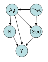 Figure 5. Example of a causal diagram showing different linkages between total N (N) and some ecological response (Y). Other circles represent percent agriculture (Ag), substrate sediment (Sed), and precipitation (Prec). Arrows indicate the direction of the hypothesized causal relationship.When using a causal diagram to choose concomitant variables, consideration can be given to recently developed criteria that identify a "deconfounding" set from a causal diagram (Morgan and Winship 2007, Ch. 3). According to this approach, a set of appropriate concomitant variables can be identified by selecting variables that "block" all "back-door" pathways linking the stressor of interest to the response variable. The following example illustrates the basic idea of blocking a pathway. Suppose one is interested in the effects of Nitrogen (N) on an ecological response variable, Y, and the causal diagram includes additional pathways (in this context, termed "back-door" paths) linking N to Y (Figure 5):
- N is linked to Agriculture (Ag) which directly affects Y.
- N is linked to Ag, which affects sedimentation (Sed), which directly
affects Y. - N is linked to Ag, which is linked to precipitation (Prec), which is linked to Sed, which directly affects Y.
Note that to identify a back-door path, we ignore the direction of causality, except that we require a causal effect on Y. Also note that this diagram is for illustrative purposes only and does not represent all possible pathways.
Given this causal diagram, we can identify variables that "block" different pathways: Pathway (1) is blocked by Ag, Pathway (2) is blocked by Ag or Sed, and Pathway (3) is blocked by Ag, Prec, or Sed. This diagram suggests that stratification on Ag alone would control for known confounders.
More formally, a deconfounding set of variables based on the back-door criterion satisfies the following criteria (Morgan and Winship 2007, p.69). First, no variable in the set is affected causally by the stressor of interest. Second, all back-door pathways connecting the stressor of interest to the biological response of interest should be blocked. To implement the second requirement, we identify all pathways in the diagram, connecting the stressor of interest to the ecological response of interest. As noted earlier, identification of pathways at this step ignores the direction of casual relationships, except that the pathways must include a causal effect on the response of interest, in addition to a direct effect on the stressor of interest. Including one or more variables from a pathway in the deconfounding set blocks the pathway.
"Collider" variables are affected causally by more than 1 variable in the pathway (e.g., Sed in Figure 5) and can complicate efforts to specify a deconfounding set. Allowing for colliders, a pathway is blocked if either the pathway includes a variable in the deconfounding set that is not a collider, or the pathway includes a collider variable that is not in the deconfounding set and not "ancestral" to a member of the deconfounding set. With regard to the last requirement, in other words, the graph does not contain a path that, following the directions of arrows, connects the collider to a variable in the deconfounding set. In our example, the single variable Sed does not block the causal pathway because Sed is a collider; however, Sed can occur in a deconfounding set that includes other, non-collider variables, which serve to block the pathway.
The back-door criterion is mathematically based, but many features are supported by intuition, an exception being the somewhat convoluted conditions for colliders. Attempts to fix the values of colliders in data analysis can result in artifactual correlation among other variables. A simple example of an ecological collider variable is the concentration of a chemical in a body of water, affected causally by measured sources X and Z. In a stratum with a restricted range of the sum X + Z, the variables are negatively correlated: Relatively high values of X must, in order for the sum to remain approximately constant, be paired with relatively low values of Z, and so on.
In theory, deconfounding sets are sufficient to eliminate confounding bias. In a given situation, multiple sets of concomitant variables may satisfy the criterion. One may wish to evaluate the sensitivity of results to different sets of concomitant variables. Also, because the approach focuses specifically on bias, satisfying the criterion is not an absolute requirement. Effects on variance can also be taken into account, in principle. For example, land-use variables that serve as sources of multiple stressors may be favored by the criterion, serving to block multiple causal pathways, possibly including stressors not adequately measured. Deconfounding sets might include (say) agricultural land use, or some stressors of agricultural origin. If biological effects of agriculture are largely accounted for by specific stressors, agriculture might be excluded, at a risk of some increase in bias.
Additional study is necessary to identify biological considerations important for application of this approach, which is mathematically based. In the mean time, the approach does identify possible pitfalls in the use of conditioning approaches, such as artifactual correlations resulting from inappropriate treatment of so-called "collider" variables.
Balancing Methodology and Propensity Scores
A propensity scores is said to be a "balancing score", a combination of the concomitant variables such that with the score fixed, the stressor is independent of concomitant variables. Stratifying on such a variable results in strata in which the stressor is approximately independent of concomitant variables that have been combined, so that stratum-specific analyses are not subject to confounding.
A balancing score achieves not only balance with respect to mean values of concomitant variables, but actually with respect to the entire multivariate distribution. That is, with the balancing score constant, a concomitant variable does not differ in variance, as well as mean values, between high and low values of a stressor. Such multivariate balance can be shown to provide robustness, in particular in case of nonlinear effects of the concomitant variables (Cochran 1965, Sec. 3.1).
Limitations of the Balancing Methodology
- The danger of inaccuracies from ignoring variables that should be taken into account likely cannot be completely eliminated. Causal analysis in the context of an incomplete causal model has been the focus of some specific method development (Morgan and Winship 2007, Ch. 6), but further study in the context of ecological causal analysis is warranted.
- In cases in which variables are closely associated, stratification on one may yield strata with inadequate variation for the stressor of interest for purposes of estimating stratum-specific stressor-response relationships. One can imagine an analysis where a stressor source such as urbanization is demonstrably important, but no specific stressor associated with the source is apparently important, once adjustments are made for the other stressors. Information on effects of the source may have some value, and more specific conclusions may require additional lines of evidence. As a rule, more specific conclusions require more data.
- Some variables should not be used for stratification, but may contribute useful information if incorporated using other methods. More variables than allowed in stratification may be incorporated based on models that accurately represent causal relationships among all causal variables. Some detailed modeling approaches that might be considered include structural equations models. A non-parametric approach is available for variables that satisfy a "front-door" criterion (Pearl 2009, Morgan and Winship 2007).
- The back-door criterion for selecting concomitant variables is based on acyclic causal diagrams: In an acyclic diagram, there is no path that departs from a variable and loops back to the variable, following the directions of arrows. This might be considered problematic for certain ecological systems, which are subject to feedbacks. In some cases, feedbacks may be eliminated when a variable is measured at a sequence of time points, by recognizing a distinct variable for each time point.
- The approach described, based on balancing scores and deconfounding sets, is general enough for application in situations where variables are correlated as a result of common causes, even when the direction of causality is not fully resolved. To apply the graphical approach for identifying a deconfounding set, correlations with unresolved causation are represented by two-headed arrows.
Regression Modeling
While a stratification approach has been emphasized, the roles of concomitant variables will often be approached in practice using regression modeling. Inferences related to one variable may be more accurate when based on a model that accurately represents the roles of multiple variables.
The statistical evidence favoring the need to incorporate a given variable in the model can be evaluated using model comparison procedures such as partial F tests, likelihood ratio tests, and Akaike or Bayesian Information Criteria (AIC, BIC).
Effective use of regression models can involve advanced issues such as variable selection, predictor interactions, collinearity, and influential observations, and error in measurement of predictions.
For some purposes, analysis of covariance (ANCOVA) can be viewed simply as regression analysis with a categorical variable coded using dummy variables. However, specific focus on the ANCOVA case has yielded insights on biases in analysis of observational data (Snedecor and Cochran 1989). ANCOVA is sometimes viewed as approximately adjusting treatment groups to common values of a covariate.
More Information
- In literature on data analysis for causal assessment, the confounding issue is often formulated as a bias in estimation of a population causal effect parameter, such as the population mean value of a response variable, if an explanatory variable, is held fixed for the entire population (e.g., Morgan and Winship 2007). In approaches based on stratification, stratum-specific causal effects may be combined over strata, weighting by population proportions, to estimate a population effect assumed similar across strata. CADDIS data analysis currently emphasizes data interpretation, especially based on graphical analysis. However, we suggest that general principles and limitations established for the objective of quantitative bias elimination can be applied more generally, when the objective is to recognize patterns that are consistent across levels of concomitant variables.
- A discussion of multiple regression in the context of estimating causal effects is given in Morgan and Winship (ibid., Chapter 5). While multiple regression is likely to be a valuable tool in a causal analysis context, naive application may fail generate unbiased estimates for some causal effects of interest.
- The graphical approach for choosing concomitant variables, for use in conditioning approaches, is due to Pearl (2009). A useful treatment of the framework with an emphasis on statistical analysis is Morgan and Winship (2007).
- Our emphasis in data analysis has been on scatterplot modifications. Additional special scatterplots of possible interest, such as partial regression plots, are discussed in regression texts such as Ryan (2009). Harrell (2002, pp. 29-30) discusses several interesting, simple scatterplot modifications.
- Additional discussion related to the use of statistical testing to assess what concomitant variables to include in an analysis is found in Breslow and Day (1980, p. 107), Mickey and Greenland (1989), Harrell (2001, p. 83), and Rothman (1986, Ch. 9).
- Much of the technical literature on statistical analysis of observational data has focused on comparing the removal of bias from concomitant variables, using strategies of stratification, matching, and regression modeling (e.g, Cochran and Rubin 1973). Methodology related to confounding and other biases is well-developed in epidemiology. One epidemiological text useful from the standpoint of data analysis is Rothman (1986). In many texts, criteria for confounding are put forward, which are to be applied to each variable separately to determine if it may cause confounding. The approach here, based on positions of variables in the causal diagram, is more recent and is viewed as incorporating insights previously recognized, but taking into account the entire causal diagram.
- Some of the strategies for evaluation of biological monitoring data can be related to strategies used in controlled laboratory experiments. In a laboratory experiment we hope to control some extraneous variables, holding their values relatively fixed throughout the experiment. In addition, randomization of experimental treatments provides some control of factors that may not have been recognized as important and may not have been measured. For observational data, options for control may be limited, but some available approaches are related to approaches used in controlled experiments.