Advanced Analyses
Controlling for Natural Variability
On this Page
- Sources of Natural Variability
- Methods for Controlling for Natural Variability
- Statistical Models of Natural Variability
In causal assessment, a test site is often compared to other sampled locations to determine whether the test site differs from expected values. However, even in the absence of any environmental stressors, stream communities vary across natural environmental gradients. This variation can occur longitudinally among reaches in a single stream drainage, spatially among stream drainages, and temporally within a single stream reach. Comparisons between test sites and other location are most informative when this natural variability is minimized or partitioned.
Sources of Natural Variability
Much of the longitudinal variation in community structure and function among reaches in a stream drainage can be related to some measure of stream size (Vannote et al. 1980). Measures of stream size can include watershed area (i.e., the catchment area above a sampling reach), stream order (Strahler 1957), distance from the source (i.e., linear distance along the stream channel from the most upstream permanent flow source to a sampling reach), stream width, stream depth, the product of stream width and depth, or average discharge. Often, watershed area is the simplest of these variables to measure.
The environmental characteristics of streams can also vary because of natural variation in regional landscapes. Such variation is often related to variation in landsurface form (i.e., physiography and geomorphology), surface geology and soils, potential natural vegetation or climate. Stream characteristics that can vary at this spatial scale include water chemistry variables, such as alkalinity, hardness, or salinity (i.e., if near to the estuarine zone); physical variables, such as temperature (i.e., particularly in relation to differences in elevation); and stream channel characteristics, such as stream slope and the dominant substrate particle size.
On a temporal scale, stream characteristics can vary with seasonal cycles or even daily cycles. Water temperature and discharge exhibit such seasonal cycles, as they vary in relation to climatic variables like air temperature and precipitation. Dissolved oxygen often exhibits a diurnal cycle with a maximum near the end of daylight and a minimum near the end of the night. Water temperature can also vary along with daily variation in air temperature. In addition to the seasonal variation, discharge can vary more stochastically in relation to individual precipitation events.
Methods for Controlling for Natural Variability
Several approaches can be used to reduce the magnitude of natural variability in the variables of interest (e.g., a biological response or a stressor of interest). Any approach that reduces variability can be useful, but the best approach may differ from one data set to another.
Sampling Design
Particularly for variables that vary seasonally, data may be used from a limited period called the index period within which temporal variation is minimized. This can also be a period when the variables of interest are most extreme and more likely to affect the biotic community. More stochastic variation can be avoided by not sampling during periods of high discharge related to storm events, unless environmental conditions during the periods of high discharge are of interest. Automatic equipment or sondes may be used to record the range of variation in variables that vary diurnally.
Classification
 Figure 1. This map shows an example of ecoregions from the mid-Atlantic region of United States, as defined by Omernik (1987). Regions with similar topography, climate and geological substrate are expected to contain streams that are similar with respect to hydrological and chemical conditions. The physical and chemical similarities presumably account for similarities in biota, and similarities in the types and magnitudes of responses to stressors.In classification, streams are grouped into ecologically similar classes, and analyses are then performed on these subsets of the data. When classification is effective, the influence of natural variables is reduced, so the differences remaining among locations and among variables are more likely the result of the stressor or stressors of interest. Classification may be based on directly relevant environmental factors, such as water temperature, that are relevant to the site or may adopt existing ecological classifications of streams or regions.
Several geographic classification systems (i.e., ecoregions, Figure 1) have been devised to identify regions that are thought to be relatively homogeneous with respect to aquatic ecosystems. Omernik (1987) delineates ecoregions based on land-surface form, potential natural vegetation, climate, soils, and predominant land use, while Bailey (1983) uses climate and potential natural vegetation. These ecoregions can be used to classify streams into groups in which expected conditions may be more homogeneous (Barbour et al. 1999, Omernik and Bailey 1997).
These classifications systems are hierarchical in that more homogeneous, smaller, higher-level ecoregion units (Level IV) are nested within consecutively larger, lower-level ecoregion units up to Level I. Until recently, Omernik’s Level III ecoregions were widely used in field research to group sites for the purpose of controlling natural variability, but Level IV ecoregions are now delineated for most of the United States. The choice of level depends on balancing two considerations. Smaller, higher-level ecoregions can be small enough that obtaining data from enough sites for analysis may be problematic, but the higher-level ecoregions may have significantly less variability, making it potentially easier to detect the effects of stressors. For example, the Little Miami River basin in Ohio is within the Level III, Eastern Cornbelt Plains ecoregion, but is divided among three Level IV ecoregions where the streams differ strongly in channel morphology and nutrient dynamics, because of their differing glacial histories (Daniel et al., 2009).
In other cases, Level III ecoregions may not differ significantly in the natural factors affecting stream structure and function [see analysis by Waite et al. (2000) of ecoregions in the mid-Atlantic Highlands, but also compare their results with those of van Sickle and Hughes (2000), McCormick et al. (2000), Rabeni and Doisy (2000), and Feminella (2000)]. In some of these cases, Level III ecoregions might be lumped, or one may consider using Level II ecoregions. Because Level II ecoregions are geographically larger, obtaining data from enough sites for analysis may be easier.
Within a region, streams may be further classified according to other sources of natural variation. Such factors could include temperature regime, stream size and drainage area, stream slope or gradient, the presence of wetlands, geomorphology, or watershed land-use. Such classification can be defined using statistical models to identify discontinuities in the values of environmental variables (e.g, classification and regression tree analysis). Standard criteria may also be used. A maximum mean monthly temperature of 20°C is often used to separate coldwater from warmwater streams. The State of Ohio uses watershed size-based classes, headwater streams (< 52 km2), wadeable streams (52 km2 to approximately 520 km2), and boatable streams (> approximately 520 km2) (Ohio EPA 1987), while U.S. EPA’s Environmental Monitoring and Assessment (EMAP) identified wadeable streams, non-wadeable streams, and great rivers (i.e., the mainstems of major rivers, such as the Ohio, Mississippi, and Missouri) (Flotemersch et al. 2006). When biogeographic data describing the distribution of aquatic species are available, they may be used to delineate ecoregions based on factors that are most relevant to freshwater species (Abell et al. 2008).
Statistical Models of Natural Variability
Predicting Environmental Conditions from Biological Observations (PECBO)
On this Page
- How do I Make these Predictions?
- How do I Use these Predictions in Causal Analysis?
- More Information
Different taxa generally require different environmental conditions to persist. If we know the environmental requirements for different taxa, we can predict environmental conditions at a site based on observations of these taxa. These biologically-based predictions can be useful in cases where environmental data are not available or are difficult to obtain. They can also provide valuable supporting evidence in a causal analysis.
The environmental requirements of different taxa can be represented with taxon-environment relationships. A taxon-environment relationship quantifies the relationship between the probability of observing a particular taxon and the value of one or more environmental variables (Figure 1). These taxon-environment relationships can be estimated from field data and then combined statistically with observations of the presence or absence of taxa at a new site to predict environmental conditions.
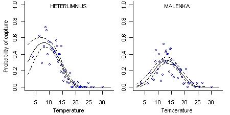 Figure 1. Taxon-environment relationships, showing the probability of capture of Heterlimnius (a riffle beetle) and Malenka (a stonefly) as a function of stream temperature. Open circles show the probability of taxon occurrence estimated from approximately 20 sites. Solid lines show the logistic regression fit to the data and dashed lines show the 90% confidence intervals about the mean line.
How do I Make these Predictions?
You can predict environmental conditions from biological observations at a site of interest if an appropriate set of taxon-environment relationships is already available, or if you have a data set that can be used to compute them.
How do I Use these Predictions in Causal Analysis?
More Information
- Environmental variables often covary (e.g., both % fine sediment and stream temperature tend to increase with decreasing elevation). Thus, when developing taxon-environment relationships, covarying environmental factors must be considered. In many cases, it is useful to model different environmental variables simultaneously.
- Technical details and programs for calculating and using taxon-environment relationships to predict environmental conditions are available as an appendix to this page.
- Taxon-environment relationships (Figure 1) can be used to identify taxa that are indicative of certain environmental conditions. However, predictions of environmental conditions as described here take into account subtle variations in the composition of the entire assemblage, and provide a more informative assessment of site conditions.
Analyzing Traits Data
On this Page
- What are the Advantages of Using this Approach?
- How do I Calculate Trait-based Metrics?
- How can Traits be Used in Causal Analysis?
- More Information
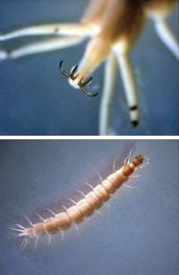 Figure 1. Beetle larvae (family Gyrinidae) with a close up of the terminal hooks.Ecological traits are attributes of an organism that provide morphological, behavioral, and functional characteristics that describe how an organism interacts with the environment. Ecological traits are inherent characteristics of individuals, e.g., the presence of suckers or hooks to maintain position in a stream (Figure 1). A trait-based approach analyzes information about ecological traits to better understand why organisms occur in particular environmental conditions.
What are the Advantages of Using this Approach?
There are two primary advantages of using a trait-based approach in biological assessment. First, trait-based descriptions of biological communities are applicable at various spatial and temporal scales. Environmental managers are asked to assess the condition of communities over a variety of spatial scales, for example by comparing condition in a local stream to general condition across a state. Descriptors based on taxonomic identity, such as the number of Ephemeroptera taxa, may be suitable for local analyses, but, unlike the taxonomic identity of individual invertebrates, responses of trait-based descriptors to changes in environmental conditions are thought to be uniform across large spatial scales. A traits-based approach, therefore, would be applicable across biogeographic boundaries. Second, a trait-based approach may provide mechanistic insight into the relationship between changes in environmental conditions and the occurrence of organisms. Better mechanistic understanding may improve the ability to predict community composition based on environmental characteristics.
How do I Calculate Trait-based Metrics?
A tool is available in CADStat that uses existing trait data from the U.S. Geological Survey (USGS) to compute trait-based metrics from observations of benthic macroinvertebrates.
How can Traits be Used in Causal Analysis?
More Information
- More background information on stream biomonitoring using species traits is available from the National Institute of Water and Atmospheric Research (see the Helpful Links box).
- Cleaned traits data and tools to calculate trait-based metrics are available in CADStat (see the Helpful Links box).
- The original trait database is publically available through USGS (see the Helpful Links box).
- Pollard AI, Yuan LL (2010) Assessing the consistency of response metrics of the invertebrate benthos: a comparison of trait- and identity-based measures. Freshwater Biology 55:1420-1429.
Propensity Score Analysis
On this Page
- What is a Propensity Score?
- How are Propensity Scores used in Causal Analysis?
- Example: Excess Nutrients
- More Information
Analysis of the role of a given stressor may be inaccurate if confounding variables are not taken into account. One method for developing a deconfounded analysis of observational data uses a type of balancing score called the propensity score.
What is a Propensity Score?
Propensity score analysis was first proposed by Rosenbaum and Rubin (1983) to infer cause and effect from studies in which experimental treatments cannot be randomly assigned to subjects. In epidemiologic research, a propensity score is an estimate of the probability that a subject would have received a ‘treatment’ (e.g., exposure to second-hand smoke), given information about his or her background. When two subjects have the same background but differ in their levels of exposure, they may be considered to have been randomly assigned to a treatment group (exposed) or control group (not exposed). Early applications tended to focus on biomedical and epidemiological issues, but applications are presently common in many disciplines.
How are Propensity Scores Used in Causal Analysis?
The original methodology dealt with a binary independent variable, e.g. comparing "treated" patients to "control" patients. In ecological causal analysis, we typically have continuous stressors rather than discrete treatment groups. In the example below, we apply stratified propensity score analysis (Rosenbaum and Rubin 1984, Imai and Van Dyk 2004), a generalization of the propensity score for continuous treatments. With this approach, the propensity score is estimated as the predicted level of a stressor, given the values of the measured covariates at a site. When used as a stratifying variable, the propensity score creates strata in which covariates are approximately independent of the stressor of interest. Regression analysis can then be used within each stratum to evaluate the effect of the stressor of interest (X) on the biological response variable (Y) without confounding by the covariates. This approach simplifies the task of minimizing multiple sources of covariation in observational data, for causal analysis.
Example: Excess Nutrients
- Estimating the propensity score
- Stratifying the dataset by the propensity score
- Evaluating the stressor-response relationship within strata
The first step, estimating the propensity score, produces the metric that will be used to stratify the dataset. Stratifying a dataset on a single variable (e.g., elevation, stream size) prior to analysis is a common technique for control of covariates, familiar to most ecologists. However, defining strata becomes increasingly difficult as the number of covariates grows. Strata of reasonable size are inevitably somewhat heterogeneous with regard to some covariates. Stratification by propensity score solves this problem via a balancing approach, in which a single metric (the propensity score) combines the effects of multiple original covariates.
In our example the stressor of interest (total nitrogen) is a continuous variable. We will calculate a propensity score for each site by modeling log-transformed total nitrogen as a linear function of the five covariates:
ps = E[log(TN)] = b0 + b1log(Area) + b2Ag + b3 Sed + b4 log(Precip) + b5 log(Cl) [Eq. 1]
where:
 Figure 1. Scatterplot of observed and predicted total nitrogen. Predicted TN is the propensity score for each sample, estimated in step 1. The vertical lines are quartiles calculated in step 2. The 4 strata defined by the propensity scores are labeled (A,B,C,D)ps = the propensity score; E[log(TN)] = the modeled expected value of log total nitrogen; Area = catchment area; Ag = the percentage of agricultural land use in the catchment; Precip = annual precipitation; Cl = chloride concentration; b0 is the fitted intercept and b1 through b5 are fitted regression coefficients.
From [Eq. 1] it can be seen that the propensity score is the predicted level of total nitrogen at a site given the values of the covariates. For a given value of the propensity score (predicted TN), the actual value of total nitrogen (TN) will vary (Figure 1).
In the second step, stratification, the dataset is stratified on the propensity score. Sites within a stratum are more similar in the values of the covariates and predicted nitrogen levels when compared with sites across the full dataset. The number of strata typically ranges from 4 to 8. Rosenbaum and Rubin (1984) state that five strata are sufficient for eliminating bias in most datasets [but see Lunceford and Davidian (2004)]. In this example we split the dataset into four strata (quartiles shown in Figure 1), each containing approximately 240 observations.
Within strata, the correlations of total nitrogen with the 5 measured covariates are significantly reduced (Table 1), an illustration of the balancing concept. It follows that a stressor response evaluation for TN is less subject to confounding, when restricted to a single stratum.
| Before: | After stratification: | |
|---|---|---|
| Covariate | r | r(min, max) |
| %Agriculture | 0.61 | (0.06, 0.39) |
| Sediment | 0.64 | (0.07, 0.13) |
| log(Area) | 0.51 | (0.01, 0.09) |
| log(Precip) | -0.51 | (0.04, 0.27) |
| log(Chloride) | 0.65 | (0.10, 0.15) |
To visualize this reduction in correlation strength, compare the correlation of nitrogen and one covariate, chloride, before and after stratification (Figures 2 and 3).
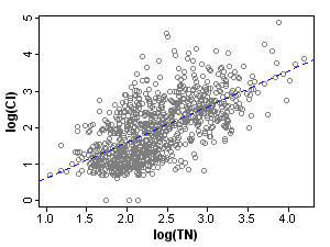 Figure 2. Scatterplot of chloride and total nitrogen in the original (unstratified) dataset. r=0.65.
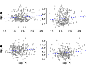 Figure 3. Scatterplot of chloride and total nitrogen in the stratified dataset. Clockwise from top left: r=0.11, r=0.11, r=0.15, r=0.10.
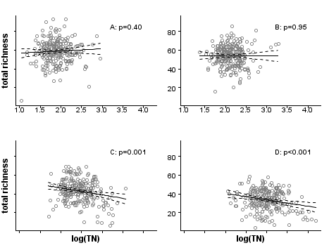 Figure 4. The effect of total nitrogen on macroinvertebrate richness varies across the 4 strata (A,B,C,D) defined by the propensity scores, shown in Figure 1. However, these results indicate that the reduction of macroinvertebrate richness may be causally related to increasing total nitrogen, after controlling for the confounding effects of watershed area, sediment, agricultural land use, precipitation, and chloride. The reader is reminded that statistical significance (p-value) may or may not indicate biological effects large enough in magnitude to be of practical concern. For more information on p-values, see the CADDIS page on interpreting statistics.The appropriate number of strata depends on the dataset. As the number of strata increases, the number of observations in each stratum decreases, reducing the sample size and statistical inferential power for analyzing the stressor response relationship stratum by stratum. However, as the number of strata increases, propensity scores within each stratum span a narrower range of values, and the covariates effects will be minimized to a greater degree.
In the third and final step, evaluating the stressor-response relationship within strata, we use regression analysis to estimate the effects of total nitrogen on macroinvertebrate richness by fitting linear regressions within each stratum (Figure 4). By using propensity scores to stratify the dataset, the bias introduced by covariates is effectively reduced, and observed effects within each stratum can be more confidently attributed to the stressor of interest. Nonparametric regressions within strata could be helpful for an exploratory approach to evaluating stressor-response relationships. In other applications, a further step would be to estimate the population effect by pooling stratum effects.
More Information
- Additional information on confounding, including a discussion of balancing and propensity scores, can be found from the Helpful Links box.
- The nutrient analysis example on this page is based on Yuan, L. L. (2010). Estimating the effects of excess nutrients on stream invertebrates from observational data. Ecological Applications 20:110-125.
Species Sensitivity Distributions (SSDs)
On this Page
- Where Can I Obtain Species Sensitivity Distributions?
- How do I Use Species Sensitivity Distributions in Causal Analysis?
- Helpful Tips
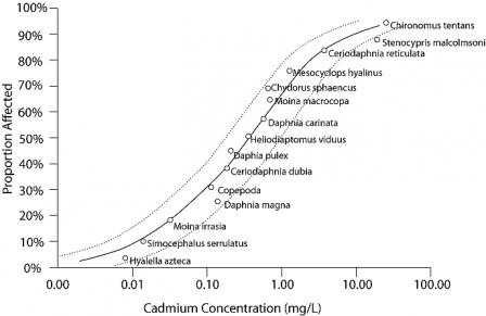
Species sensitivity distributions (SSDs) are models of the variation in sensitivity of species to a particular stressor (Posthuma et al. 2002). SSDs are generated by fitting a statistical or empirical distribution function to the proportion of species affected as a function of stressor concentration or dose. Traditionally, SSDs are created using data from single-stressor laboratory toxicity tests, such as median lethal concentrations (LC50s; see Figure 1).
Where can I Obtain Species Sensitivity Distributions?
You can create a case-specific SSD by selecting data from the literature or a database that will generate a site-relevant model. For example, since pH and hardness are important determinants for the speciation and toxicity of metals, data selected for a metals SSD should have pH and hardness similar to the site in question. If tests have been performed with local water (e.g., to derive a water-effects ratio), their results may be added to the modeled data set. Note that in general, SSDs should not be derived from fewer than five species (van Leeuwen 1990).
How do I Use Species Sensitivity Distributions in Causal Analysis?
SSDs can be used to generate predictions that may be confirmed by site data and to quantify stressor-response relationships. The interpretations discussed below, like any application of laboratory toxicity data to the field, depend on a reasonable concordance of physical, chemical, and biological conditions between the laboratory and field.
SSDs can be used to generate verified predictions using data from the case. SSDs reveal the relative sensitivities of species or other taxonomic categories. They may be used to generate predictions that certain taxa should be affected while others should be unaffected if a particular stressor is the cause of impairment. If an analysis of site data shows the predicted pattern of relative sensitivities, the prediction can be considered to be verified. Note that, to be considered a prediction, the relative sensitivities revealed by an SSD must be novel and the confirmatory data from the case must be prompted by the prediction. If the SSDs are simply consistent with the impairment (e.g., the impairment is low EPT (Ephemeroptera, Plecoptera and Trichoptera) taxa richness and the SSD shows that insects from those taxa are sensitive) no explicit prediction is verified by the data.
More frequently, SSDs provide evidence for the type of evidence stressor-response relationships from laboratory studies. By comparing site data with an SSD, they can indicate whether potentially harmful concentrations of the chemical of interest occur at the site, the magnitude of effects expected to occur at those levels, and the certainty with which an assessor may apply this information. Like all other methods of relating laboratory effects to the field, SSDs must relate the nature and magnitude of the laboratory effects to field responses. Most SSDs are based on LC50 values (i.e., concentrations at which half of the organisms die in short-term exposures) whereas most biological surveys measure the presence and the relative abundance of different species. Species may not be observed if their probability of occurrence in a sample is very low, or if they have been locally extirpated. The relationship between 50% mortality and the probability of extirpation is related to the life history traits of a species. One species may be unable to withstand even relatively small impacts on survival, growth, or reproduction; a different species may be able to persist despite episodes of 50% mortality if its reproduction rate or immigration rate is sufficiently high. Still, many chemical exposure-response curves are steep, and chemical exposures in the environment may produce more severe effects than laboratory exposures because they may be sustained or recur. For these reasons, excursions above an LC50 may well result in extirpation and be reflected in biological survey results.
Biological observations at individual sites can be compared with SSDs by expressing the biological observations as the proportion of species that have been affected at the site. First, you compare the number of species at the site to the expected number of species at that site, given habitat characteristics or the number of species in local reference sites. This comparison generates an observed/expected proportion of species, which is comparable to the inverse of the proportion of affected species (Y-axis) values of an SSD. The value of the stressor variable at the site (i.e., the X-axis variable of the SSD), is then used to compare the observed biological response with the magnitude of response predicted by the SSD.
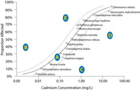 Figure 2. An SSD plot depicting five hypothetical sites (A-E) with different observed concentrations of cadmium and different proportions of species affected. Higher values on the Y-axis reflect a more severe effect.
Click image to view a larger version of Figure 2.For example, the proportion of species affected by cadmium at site A (Figure 2) is closely predicted by the model indicating that the stressor-response relationship from laboratory tests supports the candidate cause. The proportion of species affected at sites B and E are higher than predicted by the SSD model. This evidence may weaken the case for the candidate cause as the sole cause of the impairment. The proportion of species affected at sites C and D are lower than that model would predict. These results may occur when a chemical's bioavailability is low (e.g., metal ions may be bound to suspended particles), when less toxic forms of the chemical occur at the site (e.g., trivalent versus hexavalent chromium), when populations adapt or acclimate to the stressor, or when adapted species replace sensitive species. Results similar to site C may suggest that the proportion of species affected may not be an appropriate measure of impairment, because the magnitude of the measured effect is small.
Although confidence intervals are informative, they do not include uncertainty due to extrapolating from the laboratory to the field or due to variability among communities, and so they should not be used to decide whether a point is close enough to the line to be in agreement. SSD comparisons with site data are most informative when high quality site data are available, site conditions are similar to laboratory conditions with respect to relevant physical and chemical variables, and the laboratory response is relevant to the field response.
Helpful Tips
- An application of laboratory toxicity data to the field depends on a reasonable concordance of physical, chemical, and biological conditions in the laboratory and field. The data used to generate SSDs may not accurately represent toxic effects at a particular site and we recommend that an experienced aquatic ecotoxicologist help in interpreting the SSD models.
- SSDs are most easily interpreted at their extremes. If the concentrations of a chemical at an impaired site are predicted by the SSD to affect all or nearly all species, the model is consistent with the candidate cause if impairment includes effects on many species. The case for the candidate cause is weakened if the concentrations of the chemical at the site where the impairment occurs are predicted to affect no species, or only a very few.
- SSDs should be generated using data for the same type and level of effect.
- The types of taxa selected for an SSD may span several taxonomic groups, fall within a single group (e.g., arthropods or salmonids), or share certain habitat preferences (e.g., coldwater or warmwater taxa). It also may be helpful to distinguish between early and late life stages of a species, as they frequently differ in sensitivity.
- As with all analyses of secondary data, we recommend that primary sources be consulted to ensure the quality and relevance of influential data. Influential data include values that particularly influence the fitted function or that are important to the inference because they represent especially relevant site characteristics (e.g., affected taxa, stressor concentrations).
References
- Abell R, Thieme ML, Revenga C, Bryer M, Kottelat M, Bogutskaya N, Coad B, Mandrak N, Balderas SC, Bussing W, Stiassny MLJ, Skelton P, Allen GR, Unmack P, Naseka A, Ng R, Sindorf N, Robertson J, Armijo E, Higgins JV, Heibel TJ, Wikramanayake E, Olson D, Lopez HL, Reis RE, Lundberg JG, Sabaj Perez MH, Petry P (2009) Freshwater ecoregions of the world: a new map of biogeographic units for freshwater biodiversity conservation. BioScience 58:403-414.
- Bailey RG (1983) Delineation of ecosystem regions. Environmental Management 7:365-373.
- Barbour MT, Gerritsen J, Snyder BD, Stribling JB (1999) Rapid bioassessment protocols for use in wadeable streams and rivers: periphyton, benthic macroinvertebrates, and fish (2nd edition). U.S. Environmental Protection Agency, Office of Water, Washington DC. EPA 841-B-99-002.
- Daniel FB, Griffith MB, Troyer ME (2010) Influences of spatial scale and soil permeability on relationships between land cover and baseflow stream nutrient concentrations. Environmental Management 45:336-350.
- Feminella JW (2000) Correspondence between stream macroinvertebrate assemblages and four ecoregions of the southeastern USA. Journal of the North American Benthological Society 19:442-461.
- Flotemersch JE, Stribling JB, Paul MJ (2006) Concepts and approaches for the bioassessment of non-wadeable streams and rivers. U.S. Environmental Protection Agency, Office of Research and Development, National Exposure Research Laboratory, Cincinnati OH. EPA 600-R-06-127.
- Imai K, Van Dyk DA (2004) Causal inference with general treatment regimes: generalizing the propensity score. Journal of the American Statistical Association 99:854-866.
- McCormick FH, Peck DV, Larsen DP (2000) Comparison of geographic classification schemes for mid-Atlantic stream fish assemblages. Journal of the North American Benthological Society 19:385-404.
- Ohio EPA (Environmental Protection Agency) (1987) Biological Criteria for the Protection of Aquatic Life. Volume II: Users Manual for Biological Field Assessment of Ohio Surface Waters.Exit EPA Site Division of Water Quality Monitoring and Assessment, Surface Water Section, Columbus OH.
- Omernik JM (1987) Ecoregions of the conterminous United States. Annals of the Association of American Geographers 77:118-125.
- Omernik JM, Bailey RG (1997) Distinguishing between watersheds and ecoregions. Journal of the American Water Resources Association 33:935-949.
- Pollard AI, Yuan LL (2010) Assessing the consistency of response metrics of the invertebrate benthos: a comparison of trait- and identity-based measures. Freshwater Biology 55:1420-1429.
- Rabeni CR, Doisy KE (2000) Correspondence of stream benthic invertebrate assemblages to regional classification schemes in Missouri. Journal of the North American Benthological Society 19:419-428.
- Rosenbaum PR, Rubin DB (1983) The central role of the propensity score in observational studies for causal effects. Biometrika 70:41-55.
- Rosenbaum PR, Rubin DB (1984) Reducing bias in observational studies using subclassification on the propensity score. Journal of the American Statistical Association 79:516-524.
- Strahler AN (1957) Quantitative analysis of watershed geomorphology. Transactions of the American Geophysical Union 38:913-920.
- van Sickle J, Hughes RM (2000) Classification strengths of ecoregions, catchments, and geographic clusters for aquatic vertebrates. Journal of the North American Benthological Society 19:370-384.
- Vannote RL, Minshall GW, Cummins KW, Sidel JR, Cushing CE (1980) The river continuum concept. Canadian Journal of Fisheries and Aquatic Sciences 37:130-137.
- Waite IR, Herlihy AT, Larsen DP, Klemm DJ (2000) Comparing strengths of geographic and nongeographic classifications of stream benthic macroinvertebrates in the Mid-Atlantic Highlands, USA. Journal of the North American Benthological Society 19:429-441.
- Yuan LL (2010) Estimating the effects of excess nutrients on stream invertebrates from observational data. Ecological Applications 20:110-125.
Volume 4: Authors