Exploratory Data Analysis
Additional Information on Multivariate Approaches for Exploring Associations Among Stressor Variables
Basic multivariate visualization can be useful for understanding stressor correlations. Such an understanding can be helpful in dealing with issues such as confounding and collinearity that arise in evaluating multiple stressors.
For present purposes, this page emphasizes analysis of stressor variables and ignores biological response variables. Relevant resources are not reviewed comprehensively. Instead, a few basic methods are illustrated. Most of the methods considered here are discussed in Venables and Ripley (2004), and Crawley (2007), both of which are particularly useful for R implementations.
Variable Clustering
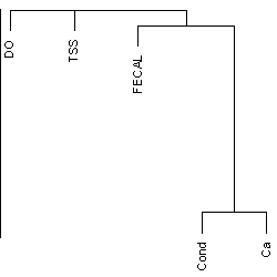 Figure 1. A dendrogram grouping variables based on squared Spearman rank correlation.Figure 1 displays clustering results using a dendrogram, a tree-like diagram. To form a dendrogram, clustering is initialized by joining the pair of variables with the highest correlation (calcium concentration [Ca] and specific conductivity [Cond], in the example). Remaining variables are incorporated in steps. Each step initiates a new cluster by combining two variables, adds a variable to an existing cluster, or combines two clusters. The varclus default decision at a given step is the so-called complete-linkage criterion: For any pair of clusters, the algorithm uses only the maximum correlation over pairs of variables with one variable in each cluster. Additional options and details are described in R on-line documentation for functions varclus and hclust (also see Venables and Ripley 2003 and Harrell 2002.)
Principal Component Analysis (PCA)
PCA is one of the most widely used multivariate statistical methods. The method is based on computation of summary variables that are weighted combinations of the original variables. (Each variable is multiplied by a weight and the weighed variables are added to form an index.) The summary variables computed in PCA are the principal components (PC), and the weights are loadings.
Figure 2 illustrates PCA based on two variables, calcium concentration (Ca) and conductivity (Cond). These variable were chosen for purely illustrative purposes, based on having a strong correlation. Each variable was transformed to logarithms and then standardized to have mean zero and variance one. Starting with the two variables Ca and Cond, PCA computes two summary variables, the PCs, which are uncorrelated. In this example, PC1 gives distance along an oblique axis where the points cluster. PC2 gives the displacement in a direction perpendicular to PC1. Evidently, the variance of PC1 is larger than the variance of PC2. The sum of variance of the two PCs is equal to the sum of variances for the original variables (in this case, 2). Thus we can say that each PC "accounts for" some percentage of variance. Indeed, in the example, the variance of PC1 scores is 1.39, so PC1 accounts for a fraction 1.39/2 = 69% of variance.
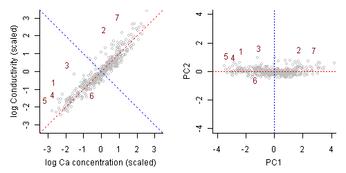 Figure 2. PCA illustrated with two variables. For each sample (represented by a point) the score for PC1 is a position along an axis where the points cluster, indicated with a red dotted line. The score for PC2 (blue dotted line) is a position in a direction perpendicular to the PC1 axis. The right-hand plot displays the same data, but with samples plotted according to PC1 and PC2, rather than Ca and cond. Selected points have been labeled with sample numbers.
More generally (for 2 or more variables) the series of PCs, denoted PC1, PC2, and so on, account for non-decreasing fractions of the original variables. (The variance of PC1 is generally larger than, perhaps occasionally equal to, the variance of PC2, which is no smaller than that of PC3, and so on. The sum of the variances of the PCs is equal to the sum of variances for the original variables.) The number of PCs is no greater than the number of original variables. In practice, one usually achieves a dimension reduction, by using a few PCs that capture most of the variance of the original variables.
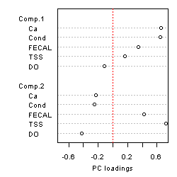 Figure 3. The interpretation of stressor associations based on principal components focuses on PC loadings. Here loadings are displayed for PC1 and PC2, from an analysis with five environmental variables: Ca = calcium concentration, Cond = conductivity, FECAL = fecal coliform concentration, TSS = total suspended solids, and DO = dissolved oxygen concentration.Results of PCA may be used in various ways in data analysis. Sometimes, a group of variables is combined into an index by computing PC1. In regression analysis, a few PCs are sometimes used in place of the original variables, to avoid a collinearity problem.
For purposes of analyzing associations among biological stressors, we emphasize interpretation of the PC loadings. Recall that these are the weights assigned to individual variables that are combined to compute a PC. Figure 3 displays loadings for a dataset that includes calcium concentration and conductivity, as for Figure 2, and three additional variables. Loadings, generated with R function princomp, are displayed using the dotchart function. A PC may be interpreted as representing the variables with loadings with largest magnitudes (positive or negative). In the example, PC1 appears to represent the strongly correlated variables Ca and Cond. PC2 appears to represent high total suspended solids (TSS) and fecal coliforms (FECAL) and low dissolved oxygen.
Jolliffe (2002) treats PCA comprehensively, including PCA derivations that do and do not involve multivariate normality , relationships to factor analysis and other multivariate methods, PCA biplots (see below), use in regression analysis, outlier-resistant methodology, choice of the number of PCs to interpret, applications to correlated data, and illustrations with applications to data from earth sciences.
Some graphical methods provide, in addition to visualization of relationships among variables, information on stressor profiles for individual sampling locations that may help the analyst to define regions or other groupings of sampling locations with distinctive stressor profiles.
Practical Defaults and Options for PCA
Running particular PCA software will usually require specifying a number of technical options. The following options are likely to generate useful results.
- PCA is often applied to standardized variables because as a rule PCA should not reflect differences in the variance of different variables, especially for variables with measurement scales that are not commensurable. (To standardize a variable, subtract the mean value and then divide by the standard deviation. After standardization, the sample mean and variance equal zero and one respectively.) Some PCA programs have an option to run the analysis based on correlations (the alternative being to use covariances). Choosing the correlation option is equivalent to running the PCA on standardized variables, so that standardized variables do not need to be computed explicitly.
- The number of PCs that the analyst should attempt to interpret is somewhat open to judgment although a number of criteria are available. Ordinarily the analyst will inspect a scree plot, in which the variances of sequential PCs (i.e., PC1, PC2,...) are graphed against indices 1, 2,... . A break in this relationship is sometimes taken to indicate the number of PCs to interpret. Another rule of thumb (for PCA applied to standardized variables) is to keep PCs that have variances no smaller than one.
- More interpretable pattern of loading are sometimes be obtained by rotation, the most common rotation approach being varimax. With varimax rotation, some loadings will be closer to zero, so that the PC can be characterized more readily in terms of variables that contribute to a given PC. A reasonable variant is to rotate only a number of PCs judged to be of interest based on the unrotated PC variances (e.g., based on a scree plot). We suggest that as a rule the analyst will evaluate loadings with and without rotation. Loadings displayed in our figure appear interpretable, without rotation.
- Applications emphasized here are exploratory in nature and do not strictly require distributional assumptions (see Jolliffe 2002). However, basic PCA is sensitive to outliers, and more useful results may sometimes be obtained by running the PCA based on rank-based or other outlier-resistant correlations, such as Spearman's correlation, as suggested by Harrell (2002, p. 66). In practice, this may involve using a correlation matrix as input to a PCA program, instead of the original data. If Pearson's correlation is used, more useful results may be obtained with variables transformed to have nearly symmetric distributions. Sometimes this is accomplished using a transformation that is fairly standard for a given variable. The variables used in our figure are concentration variables, with no non-detects. We used a logarithmic transformation, which is somewhat conventional. Similar results were obtained with Spearman's correlation (which is unaffected by transformations).
Biplots
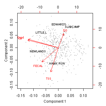 Figure 4. A biplot can be used to display information on correlations among variables, simultaneously with information on stressor profiles for individual sampling locations. For five environmental variables a PCA biplot suggests a "conductivity/Ca" axis, uncorrelated with a low DO/ high TSS axis. FECAL has a relatively higher correlation with TSS/DO than with conductivity/CA. Stream names have been included for selected sampling locations, indicating where particular samples fall in the stressor space.Certain techniques provide visualization of information on individual samples, along with information on variable correlations. Such visualization may be helpful, for example, in detecting groups of samples with similar stressor profiles, or in comparing sample locations with regard to position in a multidimensional stressor spaces. For PCA, it is common to plot the original samples as points, in a space defined by a few PCs, usually the 2-dimensional space of PC1 and PC2.
Correlations and Collinearity in Multiple Regression
In multiple regression, "collinearity" is a situation where some regressor variable can be approximated as a linear combination of other regressors. Basic regression methods cannot provide accurate inferences about the specific roles of variables that are involved in collinearity. Collinearity can result from some combination of correlations of variables in the population, or data that are few relative to the number of variables. Some regression texts emphasize that evaluation of regressor correlations early in a modeling effort can help the analyst to select a set of candidate predictors in such a way that collinearity problems are minimized (Draper and Smith 1981, Ch. 8; Harrell 2002).