Estimating Taxon-Environment Relationships: Assessing Model Fit
Assessing Model Fit
Several tools are available for assessing how closely the modeled taxon-environment relationship matches observations. Significance tests can be used to test whether the addition of a term in the model reduces the residual variance in the model by a statistically significant amount. The area under the receiver operator characteristic curve provides insight into the predictive power of the model. Also, prior to running these tests, it is useful to consider how likely your model is overfit.
Significance Tests
Statistical tests for whether the coefficients of the parametric regressions are significant are automatically listed in R by the summary command. These tests are the commonly used z-tests, but can be unreliable in certain cases. A more reliable approach for testing the significance of different terms in the regression is to apply chi-square tests. These tests compare the existing model with a set of simpler, nested models. These tests also can be used to test the significance of different non-parametric models. Statistical scripts for performing significance tests are available under the R Scripts tab of this section.
Receiver Operator Characteristic (ROC) Curves
Another useful way to quantify the performance of a model is to examine the relationship between the true positive rate and the false positive rate (Manel et al. 2001). The true positive rate is the proportion of those sites where the taxon was observed and that the model predicted the taxon as being present. The false positive rate is the proportion of those sites where the taxon was absent but that the model predicted the taxon as being present.
At a set of test sites, given the values of the environmental gradient and given a model for the taxon-environment relationship, one first computes the predicted probability of occurrence for that taxon. To compare predicted probabilities with actual observations of presence and absence, one then specifies a threshold probability above which the taxon is predicted to be present and below which the taxon is predicted to be absent.
Table 1 shows an example of comparing predicted probabilities with actual observations of presence and absence, with the threshold probability set at 0.5. The true positive rate in this case is 71/(49+71), or 0.59, and the false positive rate is 54/(195+54), or 0.22.
| Predicted absent | Predicted present | |
|---|---|---|
| Absent | 195 | 54 |
| Present | 49 | 71 |
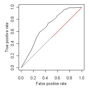 Figure 9. Receiver operator characteristic (ROC) curve for Malenka. The area under the black ROC line equals 0.8 indicating some degree of classification strength, whereas the red straight line shows a hypothetical 1:1 relationship, with area equal to 0.5 and no classification strength.As the threshold value of p increases, both false and true positive rates decrease. The trade-off can be quantified by computing false and true positive rates over a range of threshold values and plotting them against one another (Figure 9). The resulting curve is known as the receiver operating characteristic (ROC) curve, and the area under this curve provides a measure of the classification strength of the model (Manel et al. 2001). The 1:1 line indicates the position of the ROC curve for a model in which the false positive rate is the same as the true positive rate, regardless of threshold value. Such a model has no classification power, and therefore this area (0.5) is the lowest possible ROC value. The area under the ROC curve approaches 1 as classification strength increases. The minimum ROC value for an "acceptable" model varies with different studies. Statistical scripts for computing area under ROC curves are available under the R Scripts tab of this section.
Overfitting
To avoid overfitting regression models, it is generally recommended that at least 10 to 15 observations of the response variable being modeled occur in the data set for each degree of freedom in the explanatory variables (Harrell 2001).
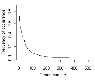 Figure 10. Distribution of frequencies of occurrence of genera collected in EMAP-West.For presence/absence data, this requirement translates into at least 10 to 15 samples with the taxon present and 10 to 15 samples with the taxon absent, per degree of freedom of the model. The single variable quadratic models described in parametric regressions have 3 degrees of freedom for each taxon. Thus, one would need 30 to 45 samples with the taxon present and 30 to 45 samples with the taxon absent. The total number of samples required depends on the overall occurrence frequency of each taxon.
Species-abundance relationships suggest that many taxa are observed infrequently and only a few are relatively common (Figure 10). Thus, the number of taxa for which regression models can be developed may be limited.
References
- Harrell FE (2001) Regression Modeling Strategies. Springer-Verlag, Inc., New York NY.
- Manel BC, Williams HC, Ormerod SJ (2001) Evaluating presence-absence models in ecology. Journal of Applied Ecology 38:921-931.