Computing Inferences: Maximum Likelihood Inferences
Maximum Likelihood Inferences
Maximum likelihood (ML) inferences use taxon-environment relationships of taxa that are present and taxa that are absent from a site to estimate the most likely environmental conditions. The simplest ML inference would use information from a single taxon.
In Figure 16, the relationship between the probability of capturing the genus Heterlimnius and stream temperature is shown. However, the vertical axis has been re-labeled to reflect the new question we are using the taxon-environment relationship to answer: what is the most likely temperature at the site, given that Heterlimnius is observed? In this case, the most likely temperature would be approximately 8° C, where the likelihood is maximized.
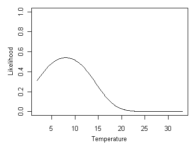 Figure 16. Likelihood curve associated with Heterlimnius being present.
What if Heterlimnius is absent from the site?
We can easily obtain the likelihood curve for an absent species by substracting the taxon-environment curve from 1 (shown in Figure 17). A stream temperature of 8° C is the least likely possibility, whereas temperatures above ~20° Care all equally likely.
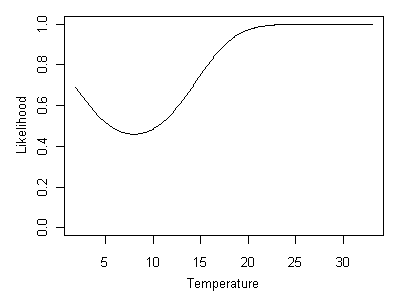 Figure 17. Likelihood curve associated with Heterlimnius being absent.
Additional taxa can be incorporated into the inference by multiplying the likelihood curves associated with each taxon. In Figure 18, the ML inference that results from both Heterlimnius and Malenka being present at a site is shown. The red line shows the product of likelihood curves for Heterlimnius and Malenka, rescaled such that its maximum value is 1. In this case, the ML inferred temperature is approximately 11° C.
 Figure 18. Likelihood curve given by Heterlimnius and Malenka being present. Heterlimnius shown as a solid line and Malenka shown a dashed line. Composite likelihood curve shown as a red line.Incorporating absences in multi-taxa inferences is straightforward. When Heterlimnius is absent and Malenka is present, ML inferred temperature is approximately 16° C (Figure 19).
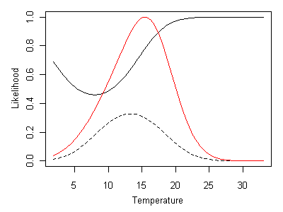 Figure 19. Likelihood curve given by Heterlimnius being absent and Malenka being present. Heterlimnius shown as a solid line and Malenka shown as a dashed line. Composite likelihood curve shown as a red line.
ML inference also offers the opportunity to quantify confidence limits on the inference, by examining the shape of the final likelihood curve.
Multivariate Models
The same approach can be used to compute inferences for multivariate taxon-environment relationships. The likelihood function for a given taxon would be a function of as many variables as used to define the taxon-environment relationship. The simultaneous effects of stream temperature and bedded fine sediment (SED) on taxon occurrences were modeled in the western U.S. These taxon-environment relationships were then used to infer temperature and SED from biological observations in Oregon. The comparison between inferences and measurements are shown in Figure 20.
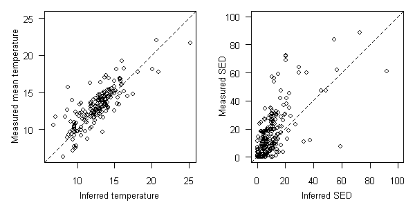 Figure 20. Comparisons between inferred and measured temperature (degrees C, left plot) and sediment (percent sand/fines, right plot) in OR. EMAP-West data used to develop taxon-environment relationships. 1:1 relationship shown as dashed line.
Identifying the Maximum Likelihood Point
As illustrated in the examples above, computing a ML inference requires that one find the point along the likelihood curve where its value is maximized (for a single variable taxon-environment relationship), or find the point within a multi-dimensional surface where likelihood is maximized (for multivariate taxon-environment relationships). In general, no analytical solution exists for this problem, and an iterative, numerical approach must be used to identify the maximum point. The function mlsolve provided in the R library bio.infer solves the maximum likelihood problem, given biological observations and a set of regression coefficients that describe taxon-environment relationships.
At the present time, the script for ML inference only works with parametric regressions. The ML solution to non-parametric taxon-environment relationships is considerably more difficult.
To use mlsolve with locally-derived taxon-environment relationships, you must use the script taxon.env (see the R Scripts tab) to analyze your local data and properly format the resulting models.
Alternatively, you can use maximum likelihood methods to infer environmental conditions using existing taxon-environment relationships from bio.infer (see the Using Existing Taxon-Environment Relationships tab).