Community Multiscale Air Quality Modeling System (CMAQ)

The Atmospheric Model Evaluation Tool

Introduction

The Atmospheric Model Evaluation Tool (AMET) was developed to aid in its evaluation of the meteorological and air quality models within the CMAQ modeling system. AMET organizes, provides consistency and speeds-up the evaluation process for operational meteorological and air quality model simulations. Although it was developed specifically to aid in the evaluation of the CMAQ modeling system, the AMET software can be adapted to work with other modeling systems.

AMET is used to pair observations and gridded model output in space and time and to evaluate the model performance for a set of predicted or diagnosed atmospheric fields. There are separate modules in AMET for evaluating meteorological and air quality model output. This separation is necessary because both the observed and predicted meteorological and air quality data are quite different, utilizing different file formats for both the observed and model data. In addition, the observed meteorological and air quality data are often obtained from networks that use different sampling protocols, which can make pairing meteorological and air quality data together difficult. One advantage of separate meteorological and air quality modules in AMET is that the modules can be installed individually, allowing a user to reduce installation time and complexity if only meteorological or air quality analysis is required.

Evaluation of model simulations, which usually includes comparing the model-predicted values against the available observed values, is critical to establishing the model’s credibility (Dennis et al., 2010). For the development of the CMAQ, evaluation of model predicted concentrations for many different atmospheric pollutants is required since the model is used to make regulatory decisions by the federal as well as state governments. The evaluation is further complicated by the requirement of evaluating the meteorological predictions that are used to provide gridded meteorological data to the CMAQ model.

Roughly a decade or so ago, CMAQ model simulations typically spanned only several weeks to a month (in some rare cases several months) and were limited spatially (for example, to the eastern half of the U.S.). The increase in computing power over time has allowed for larger model domains, longer simulation time periods and a greater number of model simulations (e.g. sensitivity and ensemble modeling studies).

Today, CMAQ simulations routinely span several months to a year and in some cases decades, and have expanded spatially to cover the continental U.S. and the Northern Hemisphere. The result is terabytes of data available for evaluation against observed data, which conventional methods of data analysis (e.g. spreadsheets) are not well suited. In addition to longer duration simulations and larger domains, the shorter wall-clock model run times have resulted in many more model simulations being performed. The increase in the duration, spatial size and number of model simulations all require greater organization and efficiency to systematically evaluate the large amounts of data being produced.

What's new in AMET Version 1.4

Streamlined database query function (AMET-AQ)
Project table species are now dynamically generated to facilitate adding new networks/species (AMET-AQ)
Improved error checking to make AMET more robust
Can now use site compare output files (csv files) to create plots, bypassing the database entirely (AMET-AQ only)
Added several new interactive plots using the R leaflet and dyGraphs libraries
Added support for the global TOAR and NOAA ESRL networks
New WRF/MPAS upper-air rawinsonde analysis
New WRF/MPAS surface shortwave radiation analysis
New WRF/MPAS PRISM analysis
New 2-m moisture time series comparison with RH
Fixed MADIS download when file is not on FTP server
Site metadata was improved to include state and elevation
Improved speed of database population

AMET-AQ Observation Data

AMET ready observation data have been made available for the years 2000 through 2017 (2017 data available are preliminary) from the CMAS Center Data Warehouse. EXIT

The network data available include: AERONET, AMON, AQS, CASTNET, CSN, FLUXNET, IMPROVE, NADP, NAPS, NOAA ESRL, SEARCH, and TOAR (other datasets may be made available in the future).

AMET Overview

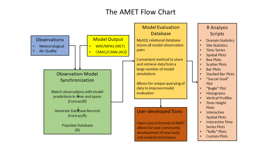
AMET is built on several open-source software packages and uses the MySQL database software to store the paired observation and model output along with various metadata. The pairing is performed by several scripts, which also insert the paired data into the MySQL database using Fortran and R programs. Finally, the analysis of the data utilizes the R statistical software package. Figure 1 presents a flow chart of the basic structure of the AMET software.

MySQL Exit
R Exit

The first step required as part of the AMET software is to pair the observed and modeled values in space and time. In the air quality module of AMET, this is accomplished through the Site Compare software. Site Compare performs matching using the nearest neighbor approach, and applies temporal averaging to the modeled data if required. In most cases, the Site Compare program is able to read the observation data files that are provided directly from the major air quality networks in the United States.

The air quality networks that Site Compare/AMET currently support are the EPA's AQS, the Chemical Speciation Network (CSN), the Interagency Monitoring of PROtected Visual Environments (IMPROVE) network, the Clean Air Status and Trends Network (CASTNET), the National Atmospheric Deposition Program (NADP) networks (AIRMON, AMON and NTN), the SouthEastern Aerosol Research and CHaracterization Study experiment (SEARCH) and the Aerosol Robotic Network (AERONET), the National Air Pollution Surveillance Program (NAPS) and the Tropospheric Ozone Assessment Report (TOAR).

The meteorological matching is performed using either bilinear interpolation or nearest neighbor. Additionally, AMET attempts to match coastal monitors with land based grid-cells as opposed to oceanic grid-cells, and both the model output and observations are considered to be on identical temporal resolutions (i.e. instantaneous values representing one hour). The meteorological module is designed to use observations from the Meteorological Assimilation Data Ingest System (MADIS). The MADIS is a widely used, comprehensive meteorological observational dataset, and requires a free subscription for access to the observation data.

MADIS Exit

Currently, the meteorological module of the latest version of AMET is designed to work with meteorological output from either the Weather Research and Forecasting (WRF; Skamarock et al., 2008) model or the Model for Prediction Across Scales (MPAS; https://mpas-dev.github.io/).

The AMET meteorological module supports evaluation of both surface and upper-air meteorological fields. The surface fields currently available in the AMET meteorological module include temperature, water vapor mixing ratio, wind speed, and wind direction. The upper-air fields available for analysis are wind speed and direction from vertical wind profilers; wind speed, direction, and potential temperature from aircraft profile (ACARS) data; and potential temperature, relative humidity, wind speed and direction from the National Weather Service balloon soundings and the model reanalysis data from the RAWINDS program.

The AMET Database

MySQL is an open-source relational database software that can used to store and quickly access large amounts of data. Aside from providing a convenient method for storing the observation-model pairs, the use of a relational database allows the entire set of data to be easily subset based on any criteria available in the database (e.g. by specific date, location or location metadata). The ability to subset the data quickly is extremely useful since model performance often varies spatially and temporally, and the spatial and temporal subsets are often different for each pollutant or chemical species. The MySQL software is free to individual users and is available for many different computing platforms.

R Statistical Package for AMET

The R project for Statistical Computing, “R”, is an open-source software for statistical computing and graphics based on the “S” language, and is available for many different computer platforms. The R software can be used through a command line interface or with the use of scripts, and contains a large number of functions for computing common statistical metrics and generating graphics (e.g. box plots and scatter plots). Additionally, the R software contains a library of modules, including a module to interface with the MySQL database software. All these features make R an attractive computational and plotting software package for AMET.

The information stored in the database is queried through for each R analysis script. Through the various commands included in the R MySQL library, the database can be queried based on any of the information stored in the database tables. For example, one could limit their data analysis to a single hour of the day, a particular day or week, or to an individual state or collection of states. The AMET scripts include instructions for performing common queries (e.g. queries based on a date range or location). However, anyone familiar with basic database queries could easily formulate their own query criteria to subset the data in any way they choose.

The AMET software already includes a collection of R scripts that perform various analyses such as computing standard statistical metrics such as bias, error and correlation; creating common statistical plots such as scatter plots and time series plots; and creating unique plots designed specifically for AMET. Table 1 lists the R scripts currently available for the AMET meteorological and air quality modules, along with a brief description of the script functions. These scripts are used to generate statistics and plot the results using the various plotting functions available in the R software. Many of the output products available in AMET are frequently used in the air quality modeling community. In addition to using the provided R scripts, the more advanced user could use these scripts as a template for creating new R scripts tailored to their particular application and analysis.

Table 1. List of R scripts currently available in the AMET meteorological and air quality modules.
Script Name	AMET Module	Description
MET AQ	Meteorological/Air Quality	Compares air quality and meteorological data. Creates a spatial plot of correlation and a time series plot of bias.
Spatial Surface Plot	Meteorological	Creates a series of maps comparing surface observations and model values. See Figure 2 for an example.
Summary Plot	Meteorological	Creates a summary plot of a series of meteorological variables. Includes time series, scatter and box plots. See Figure 3 for an example.
Met Time series	Meteorological	Creates a time series plot of temperature, mixing ratio, wind speed and direction for one or more sites. See Figure 4 for an example.
Daily Bar Plot	Meteorological	Creates a series of daily bar plots for all sites in the domain.
Profile Plot	Meteorological	Creates time-height plots of wind speed and direction profile statistics. See Figure 5 for an example.
Plot RAOB	Meteorological	Creates vertical profile plots of rawinsonde sites.
Wind Prof	Meteorological	Creates wind arrow profiles for a set of specific monitoring sites.
Box plots	Air Quality	Creates a box plot of observed and modeled quartiles.
Bugle Plot	Air Quality	Creates a “bugle plot,” which plot bias and error as a function of concentration and includes curves representing performance goals. See Figure 6 for an example.
PAVE/VERDI Overlay	Air Quality	Creates a PAVE/VERID compatible overlay file of observed values.
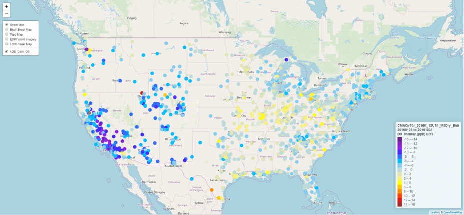
Spatial Plots	Air Quality	Numerous spatial plots available. See Figure 7 for an example. AMETv1.4 includes interactive spatial plots with map-zoom capability. See Figure 12 for an example.
Scatter Plots	Air Quality	Various scatter plots available. Includes standard model/ob scatter plot, model to model scatter plot, model skill scatter plot, etc. See Figure 8 for an example.
Soccer Plot	Air Quality	Creates a “soccer goal” plot, which plots bias verses error with performance lines in the shape of a soccer goal. See Figure 6 for an example.
Stacked Bar Plots	Air Quality	Creates a stacked bar plot of total PM_2.5 mass from networks with speciated PM_2.5 data and color codes the contribution from individual PM_2.5 species (e.g. sulfate, nitrate, ammonium, total carbon) to the total PM_2.5 mass. See Figure 9 for an example.
Stats Plots	Air Quality	Creates spatial plots of NMB, NME, FB, FE and correlation, along with a comma delimited file with various statistics.
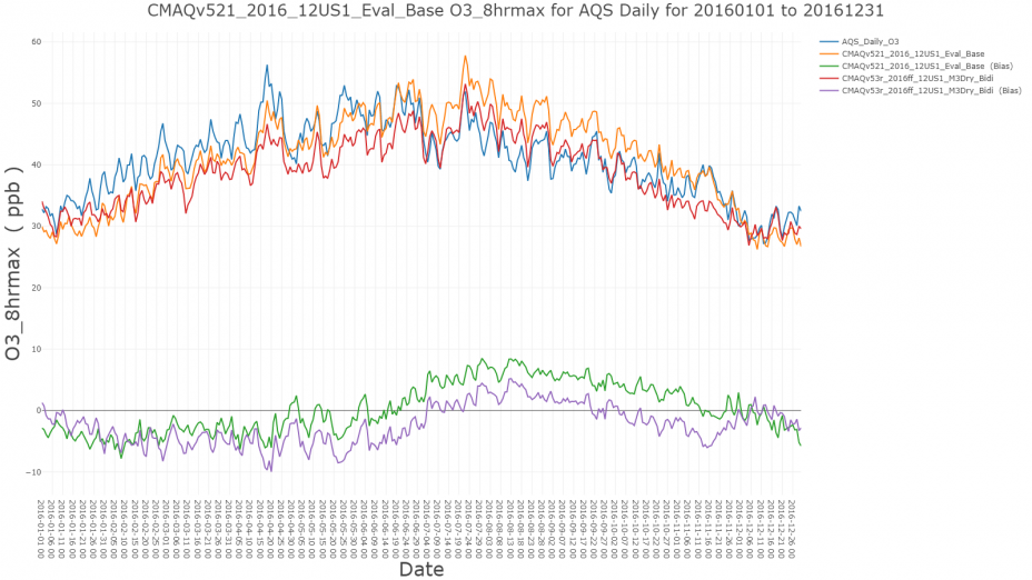
Time Series Plots	Air Quality	Various time series plots available (e.g. Model/Ob, Model/Model, time averaged). See Figure 10 for an example. AMETv1.4 includes interactive time series plots. See Figure 11 for an example.
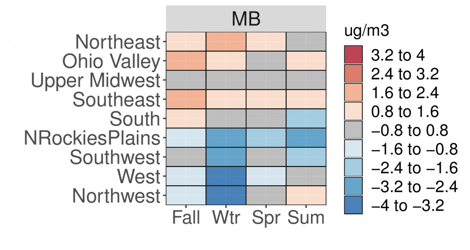
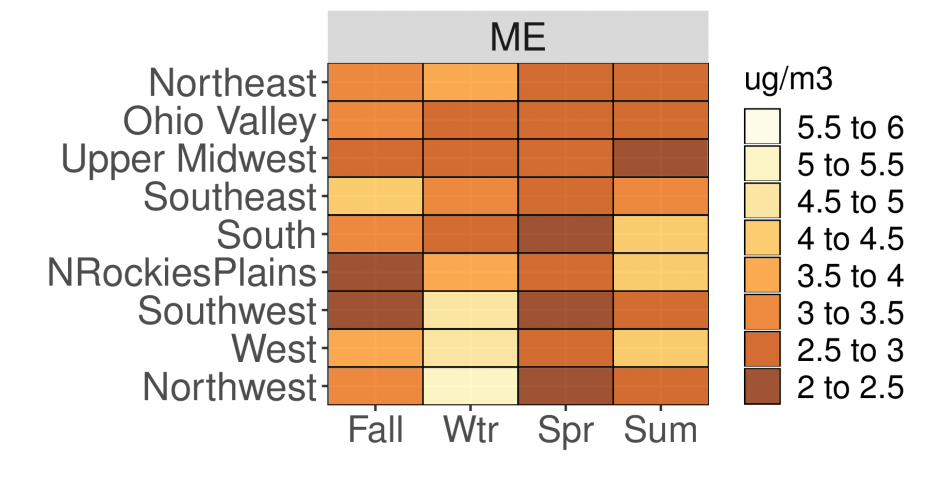
Unique Plots	Air Quality	Unique plots available such as the bugle plot, soccer goal plot and Kelly plot. See Figure 13 and Figure 14 for examples of the Kelly plots.

References

Dennis, R., Fox, T., Fuentes, M., Gilliland, A., Hanna, S., Hogrefe, C., Irwin, J., Rao, S.T., Scheffe, R., Schere, K., Steyn, D., Venkatram, A. (2010). A framework for evaluating regional-scale numerical photochemical modeling systems. Environ. Fluid Mech., 10, doi: 10.1007/s10652-009-9163-2 Exit

Skamarock, W.C., Klemp, J.B., Dudhia, J., Gill, D.O., Barker, D.M., Duda, M.G., Huang, X-Y, Wang, W., and Powers, J.G. (2008). A description of the advanced research WRF version 3. NCAR Tech Note NCAR/TN 475 STR, 125 pp, [Available from UCAR Communications, P.O. Box 3000, Boulder, CO 80307.].

Related Publications/Presentations

Appel, K.W., Gilliam, R.C., Davis, N., Zubrow, A., and Howard, S.C. (2011). Overview of the Atmospheric Model Evaluation Tool (AMET) v1.1 for evaluating meteorological and air quality models, Environ. Modell. Softw., 26(4), 434-443.

Galmarini, S., Bianconi, R., Appel, K.W., Solazzo, E., Mosca, S., Grossi, P., Moran, M., Schere, K., & Rao, S.T. (2016). ENSEMBLE and AMET: two systems and approaches to a harmonized, simplified and efficient assistance to air quality models development and evaluation. Atmos. Environ., 53, 51-59.

Appel, K.W., & Gilliam, R.C. (2008). Overview of the Atmospheric Model Evaluation Tool (AMET). 9^th Conference on Air Quality Modeling, October 9-10, 2008, RTP, NC.

Appel, K.W., & Gilliam, R.C. (2008). Overview of the Atmospheric Model Evaluation Tool (AMET). 7^th Annual CMAS Models-3 Users’ Conference, October 6-8, 2008, Chapel Hill, NC.

Additional Figures

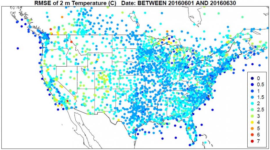Fig. 2. Sample Spatial plot from the AMET meteorological module. The plot is the root-mean-square error (RMSE) of 2-m temperature for June 2016.

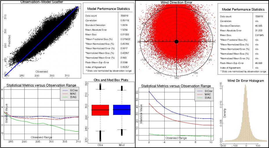Fig. 3. Sample Summary plot from the AMET meteorological module. The plot on the left is for temperature, while the plot on the right is for wind direction.

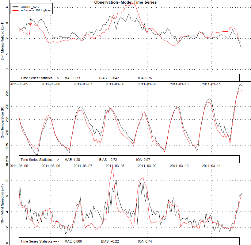Fig. 4. Sample Time Series plot from the AMET meteorological module. The top plot is for 2-meter mixing ratio, the middle for 2-meter temperature and the bottom for 10-meter wind speed.

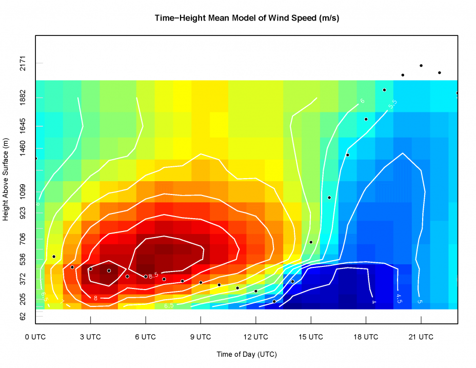Fig. 5. Sample Profile Plot from the AMET meteorological module. The color shading and white lines indicates model-predicted wind speed, while the black dots indicate the model-predicted planetary boundary layer height.

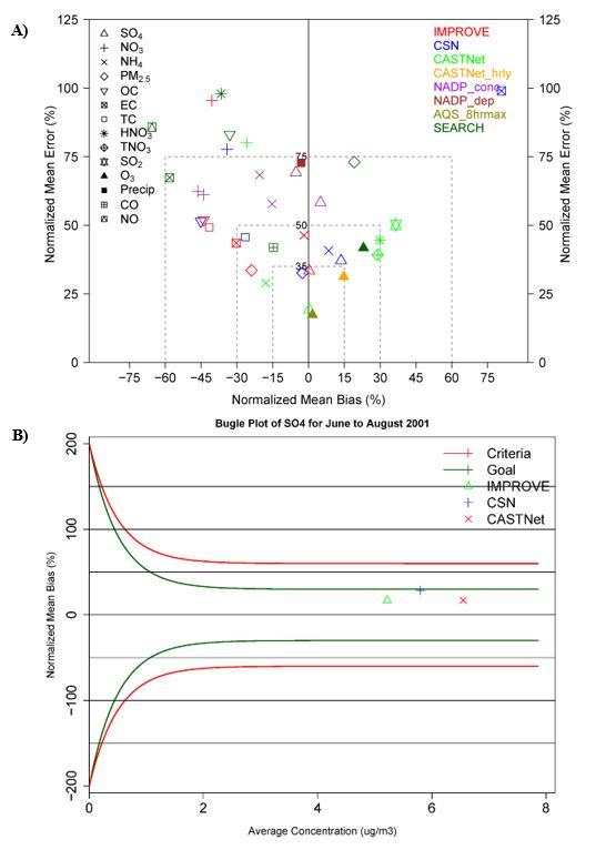Fig. 6. Sample plots from the a) Soccer Plot script and b) the Bugle Plot script from the AMET air quality module.

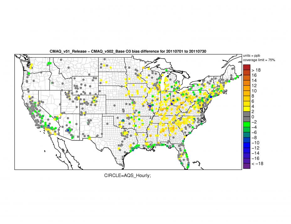Fig. 7. Sample Spatial Plot from the AMET air quality module. Shown is the difference in hourly ozone bias between two model simulations.

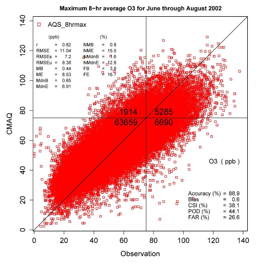Fig. 8. Example Scatter Plot for maximum daily 8-hr average ozone (shown is the Skill Scatter Plot) from the AMET air quality module.

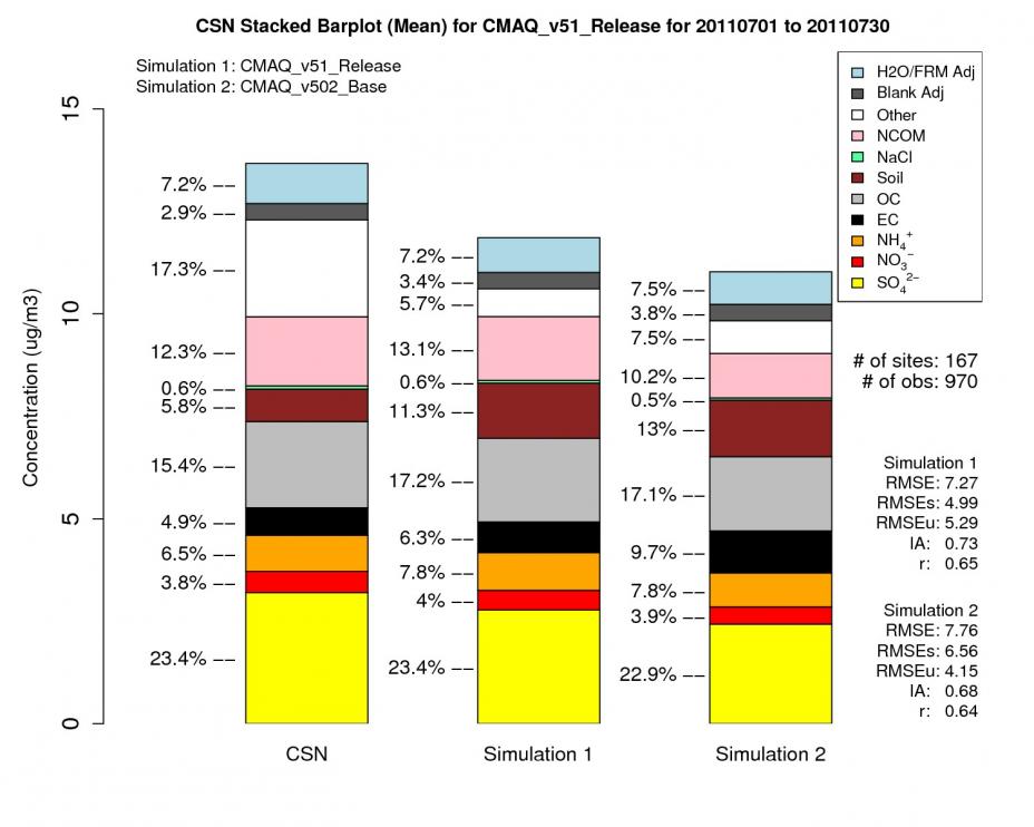Fig. 9. Sample plot from the Stacked Bar Plot script from the AMET air quality module.

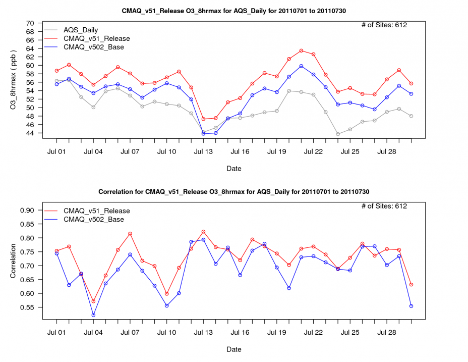Fig. 10. Example Time Series plot from the AMET air quality module. Shown on top is observed and two model simulations of ozone mixing ratio for July 2011 while the bottom plot shows the corresponding model bias.