Exposure Assessment Tools by Approaches - Exposure Reconstruction (Biomonitoring and Reverse Dosimetry)
Overview
 Exposure reconstruction is one of the three main approaches to estimating exposure. Exposure reconstruction uses internal body measurements rather than external measurements to estimate dose. (See the Indirect Estimation and Direct Measurement Modules in EPA ExpoBox for information and resources on these other approaches.)
Exposure reconstruction estimates exposure and absorbed dose using biomarker data (U.S. EPA, 2012). Stated another way, exposure reconstruction uses information collected following exposure and "downstream" of the point of exposure. In contrast, scenario evaluation and direct measurement use information collected prior to exposure and "upstream" of the point of exposure.
Successfully performing exposure reconstruction requires modeling tools such as pharmacokinetic (PK) models.
Biomonitoring data are necessary for exposure reconstruction.
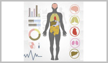
Biomonitoring involves analyzing human samples, such as tissues and body fluids, to determine contaminant or biomarker concentrations (U.S. EPA, 1992).
Biomarkers are the cellular, biochemical, analytical, or molecular measures obtained via biomonitoring from biological media (e.g., tissues, cells, fluids) that indicate exposure to a chemical (U.S. EPA, 1992).
Biomonitoring data can be combined with PK models to reconstruct or estimate the amount of chemical a person was exposed to (i.e., the exposure dose). PK models simulate the distribution and movement of chemicals within a living system. PK models can also be applied to predict an internal dose or biomarker concentration using the intake dose.
The primary benefit of reconstructing exposure using biomonitoring data is that both aggregate and cumulative exposure can be quantified. However, it may not be possible to identify specific sources or routes of exposure (e.g., inhalation, ingestion, or dermal).
Biomonitoring
Biomonitoring is the act of measuring the concentration of chemicals, their metabolites, or their byproducts in:
Biomonitoring measures the actual levels of chemicals, metabolites, or byproducts in the body.
- Tissues, such as skin and hair
- Body fluids, such as blood, saliva, semen, and breast milk
- Excreta, such as urine and feces, or
- Exhaled air
(CDC, 2009; Hays et al., 2007).
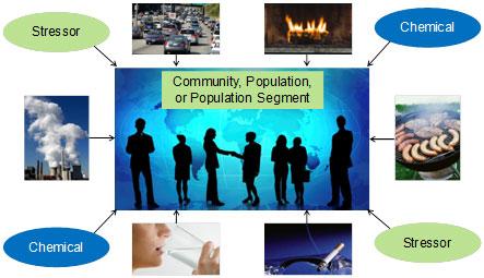
Biomonitoring data can be used to infer human exposure from multiple pathways and sources. These measurements reflect external factors that can influence both the extent of exposure for individuals or a population and their biological response to exposure (NRC, 2006; Sexton et al., 2004).
There are advantages and limitations associated with biomonitoring.
| Biomonitoring Advantages | Biomonitoring Limitations |
|---|---|
| Measures aggregate and cumulative exposure (i.e., all sources, all routes, all pathways) | Not source- or pathway-specific |
| Reflects uptake and accumulation | Requires permissions for collection of human specimens |
| Might be able to correlate internal dose with observed health effects | Difficult to interpret potential health risks |
| Can be costly |
National Health and Nutrition Examination Survey (NHANES)
The National Health and Nutrition Examination Survey (NHANES) is conducted by the Centers for Disease Control (CDC). It provides a large data set of biomonitoring data that is “designed to assess the health and nutritional status of adults and children in the United States”.
NHANES interviews and physical examinations are conducted continuously with information gathered from approximately 5,000 people each year. Interviews are used to gather information about topics including demographics, diet and exercise habits, and housing characteristics.
Physical examinations, including blood and urine samples, a cardiovascular fitness test, and dental and vision examinations, are conducted by trained medical professionals. NHANES findings are the basis for national averages and distributions for measurements like height, weight, and blood pressure (CDC, 2009).
The chemical-specific biomonitoring data collected through NHANES are available for direct download from the NHANES website. Summaries of the results are published in a series of reports referred collectively as the National Report on Human Exposure to Environmental Chemicals. NHANES data have been used to:
- Characterize body burdens,
- Determine populations with increased body burdens,
- Identify exposure levels in populations of concern,
- Establish reference or background values and identify unusually high exposures,
- Assess efforts to reduce exposure and trends over time,
- Direct research priorities, and
- Connect exposure to body burden.
The National Report on Human Exposure to Environmental Chemicals currently includes information on 246 chemicals and these data are stratified by age, race, and sex (CDC, 2012, 2009).
Because data are gathered periodically and across large population segments, trends in body burdens of chemicals for specific subpopulations can be analyzed. Health status information has also been used along with the biomonitoring data to investigate potential relationships between chemical exposure and diseases (CDC, 2009).
Survey data on health status, family history, and behaviors can be combined with data from blood and urine samples to explore relationships between exposure, external factors, and resulting body burdens. Researchers can also use health and behavior data to determine which exposure pathways are most relevant for specific chemicals based on the biomonitoring data (CDC, 2009).
Other Sources
NHANES is the most comprehensive source for human biomonitoring data in the United States. Other sources of biomonitoring data include the National Institute of Health’s (NIH) National Children’s Study, the German Environmental Survey (GerES), the German Environmental Specimen Bank (ESB), and the Canadian Health Measures Survey (CHMS).
The NIH’s National Children’s Study is an ongoing effort. With at least 100,000 children participating across the United States, it is the largest long-term study of children’s health and development. Researchers collect blood, urine, breast milk, meconium, nail, and hair samples from the children and their mothers. Biomarkers for exposure to pesticides, metals, volatile organic compounds, and other chemicals are measured.
The German Environmental Survey (GerES) examines the exposure of Germany's general population to environmental contaminants. Four GerES surveys have been conducted since 1985. The most recent survey, the German Environmental Survey for Children (GerES IV), was conducted from 2003 to 2006. It collected information from 18,000 children. Concentrations of neurotoxins (e.g., Pb, Hg), carcinogens (e.g., VOCs, PAHs, Arsenic), and other substances (e.g., PCBs) in blood and urine were measured.
In addition to GerES, Germany’s Federal Environment Agency (Umweltbundesamt) conducts other health-related monitoring including maintenance of the Environmental Specimen Bank. The Bank, archives human samples of blood, blood plasma, urine, saliva, and hair. This allows scientists to track the deposits of chemicals in humans as well as their distribution and transformation.
The Canadian Health Measures Survey (CHMS) began in 2007 to collect information about the health and lifestyles of Canadians. Its structure and survey methods parallel NHANES. Interviews and physical examinations are used to gather information for CHMS. Physical measurements, blood and urine samples, information on nutrition, health status, lifestyle, demographics, and socioeconomics are collected. CHMS is also collecting indoor air measurements and monitoring activity patterns for some study participants.
Other Sources of Biomonitoring Data
Tools
Several resources are available to risk assessors that provide information and guidance on the use of biomonitoring data.
Exposure Reconstruction
Reconstruction of exposure relies on biomarker measurements and intake and uptake predictions to estimate dose levels (U.S. EPA, 2012). There are two primary approaches for converting biomarker measurements to dose or environmental levels as recommended by NRC (2006): REVERSE DOSIMETRY and FORWARD DOSIMETRY (U.S. EPA, 2012).
Biomonitoring involves analyzing tissues (including blood and hair), body fluids, excreta, or exhaled air to determine contaminant or biomarker concentrations (U.S. EPA, 1992).
Biomarkers are cellular, biochemical, analytical, or molecular measures obtained from biological media (e.g., tissues, cells, fluids), that can indicate exposure to a chemical (U.S. EPA, 1992). A metabolite in urine, for example, may serve as a biomarker for exposure to the parent chemical.
Biomarker data, gathered through biomonitoring, can strengthen exposure assessment.
Using PK Models in Exposure Assessment: Predictive and Reconstructive Assessments
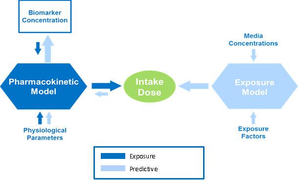
Exposure Reconstruction is illustrated by the dark blue arrows in the figure. It is the process of estimating an external exposure to a chemical that is consistent with and based on biomonitoring data. This reconstructive analysis, sometimes called reverse dosimetry, can be accomplished using pharmacokinetic (PK) models.
PK models combine data about physiological and metabolic processes with biomarker concentrations or other biomonitoring data to mathematically estimate exposure or dose. Reconstruction can happen only after exposure has taken place. It can be used to estimate exposure based on information from an effect or outcome or a target dose. The exact sources and pathways of exposure resulting in the biomarker concentration of the chemical cannot be determined by this method.
With the appropriate PK model, exposure reconstruction has the potential to provide the most accurate estimate of total exposure.
In the opposite direction, as discussed in the Indirect Estimation Module of EPA ExpoBox, an exposure model can be used to estimate intake dose based on media or exposure concentrations and exposure factors. From there, a PK model can "predict" biomarker concentrations by combining physiological parameters with intake dose, as illustrated above by the light blue arrows.
Pharmacokinetic Models
PK models provide insights into the body burdens that result from specific exposures, but require specific knowledge of model parameters and of the relationship between exposure and internal dose.
Pharmacokinetic (PK) models can be used to help characterize exposure when used in conjunction with biomonitoring data. These models relate exposure to internal dose (predictive analysis), or vice-versa to relate internal dose to exposure (reconstructive analysis) (U.S. EPA, 2006).
There are advantages and limitations to using PK models. Using PK models for exposure reconstruction is potentially a very powerful application. However, detailed input parameters for the PK model must be known for the model to be reliable. Most importantly, the relationship between exposure and dose, including bioavailability, needs to be well understood, which is not always the case.
PK models vary in complexity. The simplest PK model is a one-compartment, first order model. This assumes immediate distribution of a chemical within a single “compartment” such as blood or body lipids or even the whole body of the organism.
The creatinine correction model is an example of a simple PK model that is applicable for contaminants that are excreted in urine within hours following intake.
In comparison to these simple models, a physiologically based PK (PBPK) model is a complex, multi-compartment model. It accounts for an organism’s physiology and the chemical properties of the contaminant.
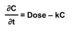
Simple
A simple one-compartment, first-order PK model estimates the change in concentration (C) in one compartment over time given a specified exposure or intake. It takes what comes in (Dose); subtracts what goes out via an elimination rate constant (k); and calculates the change in concentration of a chemical (the body burden) over time (t).
Simple models have minimal overall data requirements, but do not model the fate of the chemical in the body. They cannot, therefore, address target organ dose which is often necessary for a toxicology study. A one-compartment PK model is most often applied for contaminants that bioaccumulate in body tissues. Bioaccumulative contaminants typically have overall elimination half-lives on the order of years (e.g., lead, dioxin, DDT).
Diagram of Simple, One-Compartment Model
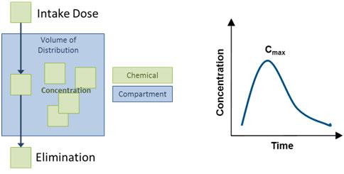
The compartment might also be referred to as the "volume of distribution", or V, and might represent the entire body or a part of the body (e.g., the blood). The elimination rate constant, k, is related to the elimination half-life of the chemical, specifically k = 0.693/half-life.
The simple one-compartment PK model can be applied in an iterative mode. This means that it can be applied in the context of a computer model structure where the key input parameters can vary over time. Another common application is to assume steady state conditions, where these inputs do not vary over time. Mathematically, this can be used to:
| Solve for Concentration given Dose | Solve for Dose given Concentration |
|---|---|
 |
 |
Creatinine Correction Model
Many contaminants do not bioaccumulate, but rather are eliminated from the body. Elimination occurs mostly by urine excretion, within a matter of hours following intake. The most common model for reconstructing dose for contaminants that are eliminated via urine is the creatinine correction model.
Muscles excrete creatinine daily in urine. Simple functions exist to estimate the expected daily creatinine excretions adjusted for sex, age, body weight, height, and race (Mage et al., 2008; Mage et al., 2004; Cockcroft and Gault, 1976).
Creatinine is measured to normalize urine concentrations. There are situations where high contaminant concentrations occur because of low urine volume not high excretion of the contaminant. Urine volume is a function of hydration, but creatinine excretion is expected to be more uniform and not a function of hydration. Therefore, a creatinine concentration tends to be more stable than a volume-based concentration.
Creatinine is regularly measured along with urine-excreted contaminants in surveys like NHANES. Contaminant concentrations are expressed in terms of mass contaminant/mass creatinine.
The creatinine correction approach can be used to estimate the daily intake of the contaminant if the exposure is ongoing, and most of the contaminant or its metabolites are excreted in urine daily.
Assuming these conditions are true, then daily contaminant excretions can be estimated using this equation:
Reconstructing dose using the creatinine correction approach is only applicable if exposure is ongoing and daily excretion is assumed to be directly correlated to daily exposure.
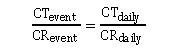
where CR is creatinine excretion and CT is the contaminant or the contaminant metabolite excretion. Rearranging this equation allows daily excretion of a contaminant (i.e., CT daily) to be calculated.
Complex
Actual exposures and human body physiology are more complicated than what is captured in a one-compartment, first-order steady-state model. The first-order model can be adapted to a temporal (unsteady-state) framework. For example, the chemical in only one compartment of the body is modeled, but the dose, rate constant, and even the volume through which the chemical is distributed can change over time.
More complex PK models account for an organism’s physiology in their equations and are called physiologically based pharmacokinetic (PBPK) models. PBPK models require parameterization to simulate the movement and fate of chemicals within the body, considering transfers between tissues and organs, metabolism, and storage.
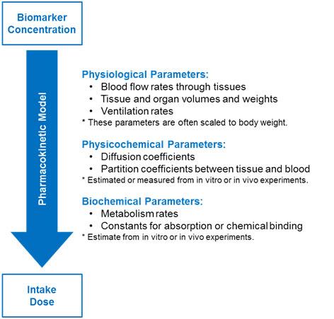
Parameters might be physiological, physiochemical, or biochemical in nature (see the figure below). There are often practical limitations to using PBPK models for exposure reconstruction. This is because of the lack of valid parameters for the numerous transfer and rate constants for human exposure scenarios.
Parameters used in a PBPK model to determine intake dose from biomarker concentration (Moir, 1999)
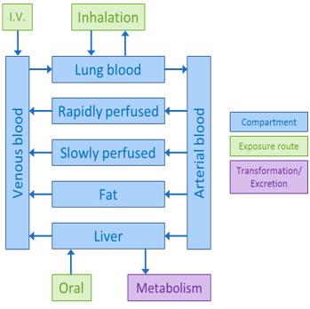
Multiple-compartment models are more complex and typically include the organs and tissues relevant for the specific chemical distribution, metabolism, or toxicity. These models might specify venous movement of blood (away from organs and back to the heart and lungs) and arterial movement of blood (away from the heart and lungs to the rest of the body).
More complex models can also describe the formation and transport of metabolites. Creating these mathematical models requires specific physiological data. For many chemicals, such data are often unavailable to build these more complex models.
Complex PBPK model adapted from pg 13 of 1,4-dioxane IRIS (U.S. EPA, 2010).
Selected Resources
- Selected References: Biomonitoring
- Selected References: Dose Reconstruction and PK Modeling
- Selected References: Creatinine Correction Approach
Selected References: Biomonitoring
- Centers for Disease Control and Prevention (CDC) (2009). Fourth National Report on Human Exposure to Environmental Chemicals (PDF) (529 pp, 6.4 MB, About PDF).
- Centers for Disease Control and Prevention (CDC) (2015). Fourth National Report on Human Exposure to Environmental Chemicals, Updated Tables.
- Clark, K; David, RM; Guinn, R; Kramarz, KW; Lampi, M; Staples, CA. 2011. Modeling human exposure to phthalate Esters: A comparison of indirect and biomonitoring estimation methods. Human and Ecological Risk Assessment: An International Journal, 17:4, 923-965.
- Clewell, HJ; Tan, YM; Campbell, JL; Andersen, ME. 2008. Quantitative interpretation of human biomonitoring data. Toxicology and Applied Pharmacology 231: 122–133.
- Hays, SM; Becker, R; Leung, HW; Aylward, LL; Pyatt, DW. (2007). Biomonitoring equivalents: A screening approach for interpreting biomonitoring results from a public health risk perspective. Regulatory Toxicology and Pharmacology. 47:96-109.
- Koch, HM; Calafat, AM. Human body burdens of chemicals used in plastic manufacture. Philosophical Transactions of the Royal Society B-Biological Sciences 2009: 364(1526): 2063-2078.
- NRC. (2006). Human biomonitoring for environmental chemicals. Washington, DC: National Academy Press Exit.
- Ott, WR. (1985). Total human exposure: An emerging science focuses on humans as receptors of environmental pollution. Environmental Science & Technology, 19, 880‐886.
- Paustenbach, D; Galbraith, D. (2006). Biomonitoring and biomarkers: Exposure assessment will never be the same. Environmental Health Perspectives, 114, 1143–1149.
- Sexton, K; Needham, LL; Pirkle, JL. (2004). Human biomonitoring of environmental chemicals: Measuring chemicals in human tissue is the "gold standard" for assessing the people’s exposure to pollution. American Scientist, 92(1), 39-45.
Selected References: Dose Reconstruction and PK Modeling
- Blancato, JN; Power, FW; Brown, RN; Dary, CD. (2006). Exposure related dose estimating model (ERDEM): A physiologically-based pharmacokinetic and pharmacodynamic (PBPK/PD) model for assessing human exposure risk. EPA/600/R-06/061.
- Egeghy, P; Lorber, M. (2010). An assessment of the exposure of Americans to perfluorooctane sulfonate: A comparison of estimated intake with values inferred from NHANES data. J. Expo Sci Environ Epidemiol 21: 150–168.
- Koch, HM; Becker, K; Wittassek, M; Seiwert, M; Angerer, J; Kolossa-Gehring, M. (2007). Di-n-butylphthalate and butylbenzylphthalate – urinary metabolite levels and estimated daily intakes: pilot study for the German Environmental Survey on children. Journal of Exposure Science and Environmental Epidemiology, 17, 378-387.
- Lorber, M. (2002). A pharmacokinetic model for estimating exposure of Americans to dioxin-like compounds in the past, present, and future. Science of the Total Environment 288:81-95.
- Lorber, M; Calafat, A. (2012). Dose reconstruction of di(2-ethylhexyl) phthalate using a simple pharmacokinetic model. Environ Health Perspect 120:1705–1710.
- Moir, D. (1999). Physiological modeling of benzo(a)pyrene pharmacokinetics in the rat. In H. Salem and S.A. Katz (Ed.), Toxicity assessment alternatives: Methods, issues, opportunities (pp. 79-95). Totawa, NJ: Humana Press.
Selected References: Creatinine Correction Approach
- Cockcroft, DW; Gault, MH. (1976). Prediction of creatinine clearance from serum creatinine. Nephron 16: 31-41.
- Mage, DT; Allen, RH; Gondy, G; Smith, W; Barr, DB; Needham, LL. (2004). Estimating Pesticide Dose from Urinary Pesticide Concentration Data by Creatinine Correction in the Third National Health and Nutrition Examination Survey (NHANES-III) Exit. J Expo Anal Environ Epidemiol 14: 457-465.
- Mage, DT; Allen, RH; Kodali, A. (2008). Creatinine Corrections for Estimating Children's and Adult's Pesticide Intake Doses in Equilibrium with Urinary Pesticide and Creatinine Concentrations Exit. J Expo Sci Environ Epidemiol 18: 360-368.
References
- CDC Research Inc. (2009). Fourth National Report on Human Exposure to Environmental Chemicals (PDF) (529 pp, 6.36 MB, About PDF).
- CDC Research Inc. (2015). Fourth National Report on Human Exposure to Environmental Chemicals, Updated Tables.
- Cockcroft, DW; Gault, MH. (1976). Prediction of creatinine clearance from serum creatinine. Nephron 16: 31-41.
- Hays, S; Becker, R; Leung, H; Aylward, L; Pyatt, D. (2007). Biomonitoring Equivalents: A Screening Approach for Interpreting Biomonitoring Results from a Public Health Risk Perspective Exit [Review]. Regul Toxicol Pharmacol 47: 96-109.
- Mage, DT; Allen, RH; Gondy, G; Smith, W; Barr, DB; Needham, LL. (2004). Estimating Pesticide Dose from Urinary Pesticide Concentration Data by Creatinine Correction in the Third National Health and Nutrition Examination Survey (NHANES-III) Exit. J Expo Anal Environ Epidemiol 14: 457-465.
- Mage, DT; Allen, RH; Kodali, A. (2008). Creatinine Corrections for Estimating Children's and Adult's Pesticide Intake Doses in Equilibrium with Urinary Pesticide and Creatinine Concentrations Exit. Journal Expo Sci Environ Epidemiol 18: 360-368.
- Moir, D. (1999). Physiological modeling of benzo(a)pyrene pharmacokinetics in the rat. In H Salem; SA Katz (Eds.), Toxicity assessment alternatives: Methods, issues, opportunities (pp. 79-95). Totowa, NJ: Humana Press Exit.
- NRC (National Research Council). (2006). Human Biomonitoring for Environmental Chemicals. Washington, DC: National Academy Press Exit.
- Sexton, K; Needham, L; Pirkle, J. (2004). Human Biomonitoring of Environmental Chemicals: Am Sci 92: 38-45 (8 pp, 2.6 MB, About PDF)Exit.
- U.S. EPA. (1992). Guidelines for Exposure Assessment [EPA Report]. (EPA/600/Z-92/001). Washington, DC.
- U.S. EPA. (2006). Approaches for the Application of Physiologically Based Pharmacokinetic (PBPK) Models and Supporting Data in Risk Assessment (Final Report) [EPA Report]. (EPA/600/R-05/043F). Washington, DC.
- U.S. EPA. (2010). Toxicological Review of 1,4-Dioxane (CAS No. 123-91-1) in Support of Summary Information on the Integrated Risk Information System (IRIS) [EPA Report]. (EPA/635/R-09/005-F). Washington, DC.
- U.S. EPA. (2012). Biomonitoring - An Exposure Science Tool for Exposure and Risk Assessment. (EPA/600/R-12/039). Washington, DC.