Estuary Data Mapper (EDM), Web Coverage Service (WCS), and Decision Support Tools
- Investigating potential water quality impacts from development, other land uses, and climate change (NOAA's Nonpoint Source Pollution and Erosion Comparison Tool, OpenNSPECT)
- Analyzing effects of sea level rise on coastal resources (Sea Level Affecting Marshes Model, SLAMM)
- Making decisions about conservation, restoration, and planning (Habitat Priority Planner). NOTE: Habitat Priority Planner has been removed from NOAA's Digital Coast site.
- Evaluating consequences of management actions on ecosystem services (Integrated Valuation of Environmental Services and Tradeoffs, InVEST)
These tools’ effectiveness can be enhanced by accessing the types of data that EDM provides. EDM uses standard Web Coverage Service Exit(WCS) queries to retrieve this data and logs an EDM session’s queries in a text file. Researchers with sufficient programming experience can use that log to start researching and crafting a command they can include in decision support tools to ingest the necessary data.
This page provides WCS examples for different types of files (tab-delimited point data, shapefile polygon/polylines, and gridded hourly data) and how those results appear in the EDM log file. Consider this page as a starting point for your own discoveries; crafting WCS queries is a trial-and-error process and each type of data carries its own idiosyncracies to either work with or work around. If you need help crafting your queries or have questions about EDM’s use of WCS commands, please contact us.
Also refer to a short list of WCS performance tips that will improve bulk data retrievals.
- Video: EDM, WCS, and Decision Support Tools
- EDM's Log File
- Using cURL for Running WCS Queries
- How EDM Retrieves Data Using WCS
- Scenario: Selecting Data Sources in EDM
- Example: Get NDBC Buoy water temperature data (type = points, format = ASCII)
- Example: Get Coastal Vulnerability Data (type = polylines, format = Shapefile)
- Example: Get CMAQ Model Nitrogen Deposition Data (type = time-stepped grid, format = binary)
- Example: Save US State Borders and Estuaries (Shapefiles, ASCII)
Video: EDM, WCS, and Decision Support Tools
The following video describes WCS commands and how they're used in EDM, illustrating many of the details described elsewhere on this page.
EDM's Log File
Each time you run EDM, it writes the WCS commands for that session into a log file called edm_out.txt. You can find EDM_out.txt in the EDM application directory.
So, the easy and practical way to learn WCS queries is to simply run EDM, retrieve data, and then read the resulting edm_out.txt file. Then, execute the same WCS queries (e.g., using a utility such as curl), redirect the result to a file, and examine the file.
There are thousands of possible different WCS queries available with rsigserver (the public WCS used by EDM and other EPA applications), and they are increasing as new data is added. Note, however, that not all available WCS queries are used by EDM; most are used by other EPA applications such as RSIG.
For assistance with WCS queries, contact EDM support.
Using cURL for Running WCS Queries
curl is an open source command line tool and library for transferring data with URL syntax, supporting DICT, FILE, FTP, FTPS, Gopher, HTTP, HTTPS, IMAP, IMAPS, LDAP, LDAPS, POP3, POP3S, RTMP, RTSP, SCP, SFTP, SMB, SMTP, SMTPS, Telnet and TFTP. curl supports SSL certificates, HTTP POST, HTTP PUT, FTP uploading, HTTP form based upload, proxies, HTTP/2, cookies, user+password authentication (Basic, Plain, Digest, CRAM-MD5, NTLM, Negotiate and Kerberos), file transfer resume, proxy tunneling and more.... curl is free and open software that compiles and runs under a wide variety of operating systems....
How EDM Retrieves Data Using WCS
For small, static data, EDM reads from “built-in” files (e.g., county borders) that are included in the downloaded EDM folder.
For large and/or time-varying data, EDM reads such data as it is streamed on-demand from specific remote Web server applications ("web services") hosted at EPA, National Oceanic and Atmospheric Administration (NOAA), US Geological Survey (USGS), and other agencies and organizations.

For example, when you select EDM’s "Retrieve and Show Selected Data" button (as shown in the screenshot above), EDM requests data from EPA's rsigserver WCS. Then, rsigserver requests data from external web services such as NOAA or USGS using commands such as:
http://nwis.waterdata.usgs.gov/nwis/dv?format=rdb&list_of_search_criteria=lat_long_bounding_box&coordinate_format=decimal_degrees&range_selection=date_range&date_format=YYYY-MM-DD&nw_longitude_va=-77.6572&nw_latitude_va=40.1987&se_longitude_va=-73.8377&se_latitude_va=36.3792&begin_date=2004-07-19&end_date=2004-07-20&index_pmcode_00300=1
The above command will stream data from its source to EDM, which displays the data in its display window.
Scenario: Selecting Data Sources in EDM
The following screenshot illustrates an EDM session. Three data sources are selected – National Data Buoy Center (NCBC) buoy data, Coastal Vulnerability risk assessment data, and CMAQ nitrogen deposition data. Also selected from the Zoom Maps tab are US State and Estuaries borders. All five data types are visualized in the display window.
The terminal window underneath is what a Mac or Linux user would see when launching EDM from a UNIX shell. The terminal window shows two ordered sets of WCS queries corresponding to the five EDM data buttons/menu selections. The first three commands retrieve and stream the data to EDM. The last two commands retrieve and save to disk the state and estuary borders.
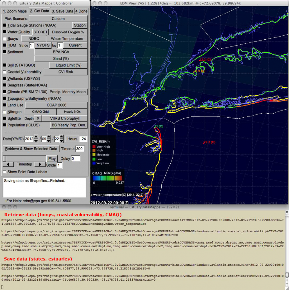
The rest of this page describes the formatting of the WCS results.
Example: Get NDBC Buoy water temperature data (type = points, format = ASCII)
The following curl command is entered in a UNIX terminal on a single line. The head command displays the first 10 lines of buoy.txt.
curl -k --silent --retry 0 -L --tcp-nodelay --max-time 3600 'https://ofmpub.epa.gov/rsig/rsigserver?SERVICE=wcs&VERSION=1.0.0&REQUEST=GetCoverage&FORMAT=ascii&TIME=2012-09-22T00:00:00Z/2012-09-22T23:59:59Z&BBOX=-74.406877,39.990239,-73.178738,41.218378&COVERAGE=erddap.ndbc.water_temperature' > buoy.txt
head buoy.txt
165
timestamp(UTC)       station_name(-)      longitude(deg)       latitude(deg) water_temperature(C)
2012-09-22T00:00:00Z      44022      -73.730000     40.880000     22.200000
2012-09-22T00:00:00Z      44065      -73.703000     40.369000     22.200000
2012-09-22T00:00:00Z      BATN6      -74.015000     40.700000     21.400000
2012-09-22T00:00:00Z      BGNN4      -74.147000     40.640000     21.600000
2012-09-22T00:00:00Z      BRHC3      -73.182000     41.173000     21.600000
2012-09-22T00:00:00Z      KPTN6      -73.765000     40.810000     21.900000
2012-09-22T00:00:00Z      SDHN4      -74.010000     40.467000     21.000000
2012-09-22T01:00:00Z      44022      -73.730000     40.880000     22.100000
...
The data returned by this command is in ASCII spreadsheet (tab-delimited) format.
The first line is the count of the data lines (not including the count and the header line).
For experienced developers, it should be straightforward to add code to an application to allocate memory then read this data into memory for display and analysis.
Example: Get Coastal Vulnerability Data (type = polylines, format = Shapefile)
The following curl command is entered in a UNIX terminal on a single line.
curl -k --silent --retry 0 -L --tcp-nodelay --max-time 3600 'https://ofmpub.epa.gov/rsig/rsigserver?SERVICE=wcs&VERSION=1.0.0&REQUEST=GetCoverage&FORMAT=bin&COVERAGE=landuse.atlantic.coastal_vulnerability&TIME=2012-09-22T00:00:00Z/2012-09-22T23:59:59Z&BBOX=-74.406877,39.990239,-73.178738,41.218378&MINDIST=0' > coastal_vulnerability.bin
Since this data is Shapefile format and Shapefile format actually consists of several files - shx, shp, and dbf - the resulting bin file is simply a one line ASCII header showing the byte count of each file (shx, shp, dbf) followed by the concatenation of the three files. The following head command displays the first line of the file.
head -1 coastal_vulnerability.bin

	coastal_vulnerability 5132 72620 89394
Shapefile-format data cannot be read directly into memory. To read the data into memory, do the following:
- Use the UNIX head command to display the one-line header
- Shunt the streamed bytes to each of the three files (shx, shp, dbf)
- Use an API library (such as the open source C shapefile libraryExit) to read the files into memory for display.
Example: Get CMAQ Model Nitrogen Deposition Data (type = time-stepped grid, format = binary)
The following curl command is entered in a UNIX terminal on a single line.
curl -k --silent --retry 0 -L --tcp-nodelay --max-time 3600 'https://ofmpub.epa.gov/rsig/rsigserver?SERVICE=wcs&VERSION=1.0.0&REQUEST=GetCoverage&FORMAT=xdr&COVERAGE=cmaq.amad.conus.drydep.no,cmaq.amad.conus.drydep.no2,cmaq.amad.conus.drydep.no3,cmaq.amad.conus.wetdep1.no,cmaq.amad.conus.wetdep1.no2,cmaq.amad.conus.wetdep1.no3&TIME=2012-09-22T00:00:00Z/2012-09-22T23:59:59Z&BBOX=-74.406877,39.990239,-73.178738,41.218378,1,1' > cmaq.xdr
CMAQ data is gridded and time-varying (hourly) so an efficient portable binary format called XDR - with an ASCII header - is used. The following head command lists the XDR file's first 17 lines.
head -17 cmaq.xdr
SUBSET 9.0 CMAQ

	12US1

	https://19january2021snapshot.epa.gov/heasd/research/cdc.html,CMAQSubset
2012-09-22T00:00:00-0000

	# data dimensions: timesteps variables layers rows columns:

	24 9 1 14 12
# subset indices (0-based time, 1-based layer/row/column): first-timestep last-timestep first-layer last-layer first-row last-row first-column last-column:

	0 23 1 1 164 177 369 380

	# Variable names:
LONGITUDE LATITUDE ELEVATION NO NO2 NO3 NO NO2 NO3

	# Variable units:

	deg deg m kg/hectare kg/hectare kg/hectare kg/hectare kg/hectare kg/hectare
# lcc projection: lat_1 lat_2 lat_0 lon_0 major_semiaxis minor_semiaxis

	33 45 40 -97 6.37e+06 6.37e+06

	# Grid: ncols nrows xorig yorig xcell ycell vgtyp vgtop vglvls[2]:
459 299 -2.556e+06 -1.728e+06 12000 12000 7 5000 1 0.9975

	# IEEE-754 32-bit reals data[variables][timesteps][layers][rows][columns]:
The big-endian IEEE-754 format data array follows the 17-line ASCII header. It is efficient and straightforward to allocate memory and read the data (rotating the 4-byte words on little-endian platforms) into memory, etc.
Note the LONGITUDE-LATITUDE-ELEVATION coordinates are for the center of each grid cell. The grid cells are contiguous squares in Lambert Conformal Conic space.
The above header contains the parameters necessary to construct the grid cell corners for proper display. However—you will need code for map projections. Refer to the Community Modeling and Analysis (CMAS) site’s documentation for details on defining horizontal and vertical grids and coordinates for Models-3.
Example: Save US State Borders and Estuaries (Shapefiles and ASCII)
The following WCS calls are issued when EDM saves data as Shapefile format and displays the resulting maps. The resulting Shapefiles are high-resolution and clipped to the view shown in the EDM display. Each curl command is entered on a single line.
curl -k --silent --retry 0 -L --tcp-nodelay --max-time 3600 'https://ofmpub.epa.gov/rsig/rsigserver?SERVICE=wcs&VERSION=1.0.0&REQUEST=GetCoverage&FORMAT=bin&COVERAGE=landuse.atlantic.states&TIME=2012-09-22T00:00:00Z/2012-09-22T23:59:59Z&BBOX=-74.406877,39.990239,-73.178738,41.218378&MINDIST=0' > states.bin
curl -k --silent --retry 0 -L --tcp-nodelay --max-time 3600 'https://ofmpub.epa.gov/rsig/rsigserver?SERVICE=wcs&VERSION=1.0.0&REQUEST=GetCoverage&FORMAT=bin&COVERAGE=landuse.atlantic.estuaries&TIME=2012-09-22T00:00:00Z/2012-09-22T23:59:59Z&BBOX=-74.406877,39.990239,-73.178738,41.218378&MINDIST=0' > estuaries.bin
Note how all of the WCS queries on this page differ in the COVERAGE option, which specifies the named data being retrieved, and the FORMAT option (which depends on the data type), and possibly other “custom options” such as MINDIST.
When saving data as Shapefile format, the following set of files are written:
ls -l coastal_vulnerability*

	-rw-rw-r--  1 plessel  staff  93765 Apr  6 18:50 coastal_vulnerability.dbf

	-rw-rw-r--  1 plessel  staff    167 Apr  6 18:50 coastal_vulnerability.prj

	-rw-rw-r--  1 plessel  staff  76652 Apr  6 18:50 coastal_vulnerability.shp

	-rw-rw-r--  1 plessel  staff   5380 Apr  6 18:50 coastal_vulnerability.shx

	-rw-rw-r--  1 plessel  staff  83650 Apr  6 18:50 coastal_vulnerability.txt

	-rw-rw-r--  1 plessel  staff  13887 Apr  6 18:50 coastal_vulnerability_atlantic.xml
In addition to the required set of Shapefiles (shp, shx, dbf, prj), a metadata file (xml) is written and also a tab-delimited text version of the dbf file, which is easier to read into non-GIS applications:
head coastal_vulnerability.txt

	LENGTH_KM    CVI    CVI_RANK    CVI_RISK    MEANWAVE_M    WAVE_RANK    WAVE_RISK    MEANTIDE_M    TIDE_RANK    TIDE_RISK    SLRISE_MMY    SL_RANK    SL_RISK    SLOPE_PCNT    SLOPE_RANK    SLOPE_RISK    EROACC_MYR    EROACCRANK    EROACCRISK    GEOMO_RANK    GEOMO_RISK

	0.306200    3.873000    1    Low    0.900000    3    Moderate    2.050000    3    Moderate    2.000000    2    Low    0.263200    1    Very Low    2.100000    1    Very Low    5    Very High

	1.030700    3.464100    1    Low    0.900000    3    Moderate    2.050000    3    Moderate    2.000000    2    Low    0.263200    1    Very Low    2.100000    1    Very Low    4    High

	0.401300    3.873000    1    Low    0.900000    3    Moderate    2.050000    3    Moderate    2.000000    2    Low    0.263200    1    Very Low    2.100000    1    Very Low    5    Very High

	1.047700    3.873000    1    Low    0.900000    3    Moderate    2.050000    3    Moderate    2.000000    2    Low    0.268800    1    Very Low    2.100000    1    Very Low    5    Very High

	0.054500    3.873000    1    Low    0.900000    3    Moderate    2.050000    3    Moderate    2.000000    2    Low    0.263200    1    Very Low    2.100000    1    Very Low    5    Very High

	1.608700    3.464100    1    Low    0.900000    3    Moderate    2.050000    3    Moderate    2.000000    2    Low    0.263200    1    Very Low    2.100000    1    Very Low    4    High

	3.180600    3.464100    1    Low    0.900000    3    Moderate    2.050000    3    Moderate    2.000000    2    Low    0.263200    1    Very Low    2.100000    1    Very Low    4    High

	0.237200    3.464100    1    Low    0.900000    3    Moderate    2.050000    3    Moderate    2.000000    2    Low    0.252700    1    Very Low    2.100000    1    Very Low    4    High

	0.190100    3.464100    1    Low    0.900000    3    Moderate    2.050000    3    Moderate    2.000000    2    Low    0.252700    1    Very Low    2.100000    1    Very Low    4    High