Basic Principles & Issues
- Establish whether biological or environmental test site conditions differ from expectations.
- Help interpret estimates of stressor-response relationships from larger, regional datasets.
- Evaluate whether stressor-response relationships are consistent among regions, study years, or species
- Determine whether one can account for biological effects of a land-use variable with proximate stressor measurements.
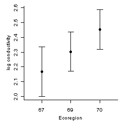 Figure 1. Confidence intervals are useful for comparison of parameter estimates, accounting for statistical error in estimation.In causal analysis, significance tests and confidence intervals can be used to:
A confidence interval provides a range for a parameter, within which values can be considered in reasonable agreement with data. Confidence intervals take into account the quantity and variability of data (Figure 1). Statistical tests can help avoid over-interpretation of noisy data by focusing analysis on effects that are unlikely attributable to data variability.
Analysts should consider the possibility that some samples in a dataset may not actually provide independent evidence because samples taken relatively close together in space or time are to some degree redundant. Measurements also may occur as clusters, with a tendency for less variation within than among clusters. For example, a study involving chlorophyll concentration in lakes may involve multiple lakes, and samples at multiple locations in each lake. In this case, samples from each lake are "clusters".
If individual samples depend strongly on one another, use of standard statistical methods that assume independence (e.g., confidence intervals) may result in greater confidence in the strength of conclusions than is actually justified by the evidence in the data.
These concerns are all associated with the technical topic of autocorrelation, or the correlation of repeated measurements on the same variable. In ecology, similar concerns may be discussed under the topic of pseudoreplication. When analyzing biomonitoring data we are most often concerned with positive spatial autocorrelation, in which measurements tend to be similar when taken from locations close together. A simple example of autocorrelation in a stream is the likelihood that conditions downstream are not independent of conditions upstream.
The first line of defense against autocorrelation problems is familiarity with the study design, along with an understanding of variation occurring on different spatial and temporal scales at the sample sites. These insights may be sufficient to identify data that are adequately independent. For example, if morphology of a stream can be described as an alternation of riffles and pools, the analyst might somehow obtain a single value for each riffle or pool, perhaps by averaging sample measurements from the same riffle or pool.
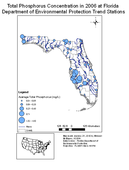 Figure 2. Total phosphorus concentrations from water samples across Florida (size of symbol is proportional to concentration).Since autocorrelation is generally present in environmental data on some scale, we emphasize graphical evaluation. Any mapping approach that can reveal a tendency for clustering of relatively high or relative low values may be effective in revealing spatial autocorrelation. For example, a map of total phosphorus concentrations in Florida suggests a cluster of high phosphorus measurements in the central western portion of the peninsula (Figure 2). Specialized graphical techniques like the variogram, discussed in the supplemental information below, can be helpful for identifying a minimum spatial or temporal separation, such that measurements will be practically uncorrelated. Statistical tests for spatial and temporal autocorrelation also are available. The usual issues in correct use of statistical tests should be kept in mind. That is, for any given level of autocorrelation, the chance of a statistically significant test will depend on sample size. Graphical techniques parallel to those for use in diagnosing spatial autocorrelation also are available for temporal autocorrelation (e.g., for use when evaluating the time series for an individual monitoring station).
If autocorrelation is judged to be important for evaluation of a given data set, based on statistical tests or graphical evaluation, relatively simple approaches may be considered appropriate for taking autocorrelation into account, in the analysis of data. Temporal correlation can be eliminated by separate analysis of "time-slices", such as individual years of biomonitoring data collection. Results for individual years may be compared using confidence intervals for effect indices. For some purposes clustered data may be reduced to a single summary statistic, for example (in the lake example) a mean value for each lake. (Note though, that we may then lose the ability to evaluate stressors that vary within lakes!)
A significant amount of statistical literature relates to how autocorrelation can be incorporated into regression models (see Additional Information on Autocorrelated Data in the Helpful Links). For modeling a times series for a single site, some relatively simple approaches involve use of lagged X variables. The analyst may, however, opt for relatively advanced multilevel models, which may allow for various patterns of autocorrelation, variation on multiple spatial scales, simultaneous modeling of data for multiple years, and stressor that vary within as well as between sites. Participation of a statistician for advanced analyses may be helpful.
The effect of a stressor on a measure of biological condition (i.e., the stressor-response relationship) may be misunderstood if other environmental variables or stressors that may affect the biological measure are ignored. In many cases, a simple relationship observed between a measure of biological condition and a single stressor may reflect the effects of additional stressors. For example, increased urban land use encompasses many different stressors (e.g., increased flow flashiness, increased concentrations of different pollutants, and degraded physical habitat), all of which can influence the aquatic biological community.
Analyses to estimate stressor-response relationships often must take measures to avoid attributing biological effects to a single stressor when observed effects are as readily attributable to simultaneous exposure to multiple, associated stressors. This issue is particularly important when estimating stressor-response relationships from large, regional data sets, in which multiple, associated stressors are common.
Identifying Concomitant Variables
One Approach for Controlling for Confounding Variables
For a basic data analysis tool that can address confounding to some degree, we emphasize scatterplots in combination with stratification. Stratification breaks the dataset into subsets (i.e., strata) that are relatively homogeneous with respect to one or more concomitant variables. If there is adequate variation within strata for the stressor of interest, one can evaluate the stressor-response relationship with concomitant variables approximately fixed, minimizing their influence on the estimated relationship. In a scatterplot, the strata may be labeled distinctively. A related approach is to use special symbols to flag points in the scatterplot that have relatively extreme values of concomitant variables.
We illustrate the use of stratification using data from streams of the western United States, in which we are interested in estimating the effects of total nitrogen (TN) on total macroinvertebrate richness. TN and percent substrate sand/fines (SED) are strongly correlated (r = 0.65), and so the bivariate relationship we would estimate between TN and total richness may be confounded by SED. To control for the effects of SED, we first break the dataset into 6 strata, defined by SED values (Table 1).
Table 1. Percent substrate sand/fines (SED) in different strata. Column labeled as "r" shows the correlation coefficient between total nitrogen and SED within each stratum.
| Stratum | SED (%) | r |
|---|---|---|
| 1 | 0 - 7 | 0.03 |
| 2 | 8 - 14 | 0.12 |
| 3 | 15 - 28 | 0.08 |
| 4 | 29 - 46 | 0.25 |
| 5 | 47 - 76 | 0.09 |
| 6 | 77 - 100 | 0.15 |
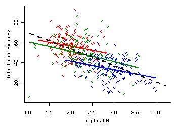 Figure 3. Example of use of stratification to control for confounding. Colors correspond to different strata based on SED values (Table 1). For clarity, only Stratum 1 (red), Stratum 4 (green), and Stratum 6 (blue) are shown. Colored lines indicate linear regression fit within each stratum. Dashed black line shows linear regression fit using full data set.Within each stratum, the strength of correlation between SED and TN is greatly reduced (Table 1), and thus, the potential confounding effects of SED on the estimate effect of TN on total richness is also reduced. One could then use regression analysis within each stratum to estimate the TN-total richness relationship (Figure 3). In this example, the slope of the relationship between TN and total richness is similar across strata (colored lines), but noticeably less steep than the slope estimated using the full data set (black dashed line). This difference suggests that SED does indeed bias the simple estimate of relationship between TN and total richness using the full data set.
If concomitant variables (e.g., other stressors, sources) are strongly correlated with the stressor of interest in the available data, the specific roles of individual stressors may be difficult to evaluate. Alternatively, a group of correlated stressor variables may be combined using some index. For example, concentrations of multiple toxic metals might be combined using a simple concentration addition model or a more mechanistic biotic ligand model. More definite conclusions about the roles of specific stressors might depend on additional types of information. Methods for evaluating associations of stressor variables may be helpful in planning an informative analysis.
More Information
A useful modification of this stratification approach can be based on propensity scores. Propensity scores combine multiple concomitant variables into a single variable that can be treated in the same way as a single concomitant variable in various approaches to data analysis.
Details regarding statistical approaches for identifying potential confounding variables and for controlling their effects can be found on the page Additional Information on Confounding, available from the Helpful Links box.
- Bivand RS, Pebesma E, Gomez-Rubio V (2008) Applied Spatial Data Analysis with R. Springer, New York NY.
- Bolker BM (2008) Ecological Models and Data in R. Princeton University Press, Princeton NJ.
- Breslow NE, Day NE (1980) The Analysis of Case-Control Studies. World Health Organization, Lyon, France.
- Burnham KP, Anderson DR (2002) Model Selection and Multimodal Inference: A Practical Information-Theoretic Approach (2nd edition). Springer-Verlag, New York NY.
- Chatfield C (1975) The Analysis of Time Series: Theory and Practice. Chapman and Hall, London UK.
- Cochran WG (1965) The planning of observational studies of human population (with Discussion). Journal of the Royal Statistical Society A 128:134-155.
- Cochran WG (1968) The effectiveness of adjustment by subclassification in removing bias in observational studies. Biometrics 24:295-313.
- Cochran WG, Rubin DB (1973) Controlling bias in observational studies: a review. Sankhya A 35:417-446.
- Cox DR (2006) Statistical Inference. Chapman & Hall, New York NY.
- Cox DR, Hinkley DV (1974) Theoretical Statistics. Chapman & Hall, New York NY.
- Crawley MJ (2007) The R Book. Wiley, New York NY.
- Dales LG, Ury HK (1978) An improper use of statistical significance testing in studying covariables. International Journal of Epidemiology 7:373-375.
- Dormann CF, McPherson JM, Araujo MB, Bivand R, Bolliger J et al. [17 authors] (2007) Methods to account for spatial autocorrelation in the analysis of species distributional data: a review. Ecography 30:609-628.
- Fisher RA (2000) Mathematics of a lady tasting tea [first published 1956]. in: J.R. Newman (Eds). The World of Mathematics. Dover Publications, Mineola NY.
- Gilbert RO (1987) Statistical Methods for Environmental Pollution Monitoring. Van Nostrand Reinhold, New York NY.
- Greenland S (1989) Modeling and variable selection in epidemiological analysis. American Journal of Public Health 79:340-349.
- Harrell FE (2001) Regression Modeling Strategies. Springer-Verlag, Inc., New York NY.
- Hinklemann K, Kempthorne O (1994) Design and Analysis of Experiments. Volume 1. Introduction to Experimental Designs. Wiley, New York NY.
- Hoenig JM, Heisey DM (2001) The abuse of power: the pervasive fallacy of power calculations for data analysis. The American Statistician 55:1-6.
- Hurlbert SH (1984) Pseudoreplication and the design of ecological field experiments. Ecological Monographs 54:187-211.
- Littell R, Milliken G, Stroup W, Wolfinger R, Schabenberger O (2006) SAS for Mixed Models (2nd edition). SAS Institute Inc., Cary NC.
- Little RJ (2004) To model or not to model: competing modes of inference for finite population sampling. Journal of the American Statistical Association 99:546-556.
- Mickey RM, Greenland S (1989) The impact of concomitant variable selection criteria on effect estimation. American Journal of Epidemiology 129:125-137.
- Miller RG (1997) Beyond ANOVA: Basics of Applied Statistics. Chapman and Hall/CRC, New York NY.
- Morgan SL, Winship C (2007) Counterfactuals and Causal Inference. Cambridge University Press, New York.
- Pearl J (2009) Causality: Models, Reasoning, and Inference. Cambridge University Press, New York.
- Pinhiero JC, Bates DM (2000) Mixed-Effects Models in S and S-PLUS. Springer, New York NY.
- Qian SS (2010) Environmental and Ecological Statistics with R. CRC Press, Boca Raton FL.
- Ramsey FL, Schafer DW (2002) The Statistical Sleuth: A Course in Methods of Data Analysis. Duxbury, Pacific Grove CA.
- Rothman KJ (1986) Modern Epidemiology. Little, Brown, and Co., Boston.
- Ryan, TP (2009) Modern Regression Methods. Wiley, New York.
- Salsburg D (2001) The Lady Tasting Tea: How Statistics Revolutionized Science in the Twentieth Century. W.H. Freeman and Company, New York NY.
- Schabenberger FJ, Pierce, FJ (2002) Contemporary Statistical Methods for the Plant and Soil Sciences. CRC Press, New York.
- Snedecor GW, Cochran WG (1989) Statistical Methods. Iowa State University Press, Ames IA.
- Sokal RR, Rohlf FJ (1995) Biometry (3rd edition). Freeman, New York NY.
- Stunkard CL (1994) Tests of proportional means for mesocosm studies. Pp. 71-84 in: Graney RL, Kennedy JH, Rodgers JH Jr. (Eds). Aquatic Mesocosm Studies in Ecological Risk Assessment. CRC Press, Boca Raton FL.
- Venables WN, Ripley BD (2004) Modern Applied Statistics with S (4th edition). Springer, New York NY.
- Waller LA, Gotway CA (2004) Applied Spatial Statistics for Public Health Data. John Wiley and Sons, New York NY.
- Zuur AF, Ieno EN, Walker N, Saveliev AA, Smith GM (2009) Mixed Effects Models and Extensions in Ecology with R. Springer, New York.