Non-Parametric Regressions

Many researchers have noted that unimodal relationships are unlikely for all taxa across all gradients (Austin and Meyers 1996, Oksanen and Minchin 2002). To address this issue, a modeling approach that requires only that the modeled function vary smoothly and slowly over the modeled range is often used. Here, the distribution of a given taxon is modeled in Equation 8:

EQUATION 8 where p is the probability of occurrence of the taxon of interest, s₀ is a constant, and s represents a nonparametric smooth curve that is fit through the data.

The locations of the mean responses for each point along a nonparametric curve, s, are determined through an iterative procedure that uses data in a local neighborhood around each point. The local nature of the fit differs fundamentally from that of a parametric model, which computes a best fit for the entire set of data. Thus, nonparametric responses can capture smaller scale variations in response (Figure 7). Near an edge of the domain, though, less data are available on one side of the point of interest, and increasing amounts of data must be drawn from within the sampled range. Therefore, the width of the neighborhood broadens at the extremes of the environmental gradient, and the fit is less local than in the center of the domain (Hastie and Tibshirani 1999).

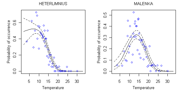Figure 7. Relationship between probability of occurrence and stream temperature (degrees C) for Heterlimnius and Malenka using a nonparametric model.The solid line shows the mean relationship between probability of occurrence and temperature. Dotted lines indicate the estimated 90% confidence limits about the location of the regression curve. Each open circle represents the average occurrence probability in approximately 20 samples surrounding the indicated temperature.

A commonly used method for fitting nonparametric curves is known as the generalized additive model (GAM) (Hastie and Tibshirani 1999). This method allows for more than one explanatory variable, each associated with its own nonparametric smooth curve.

The flexibility of nonparametric regressions also complicates this method's use because there are no parameters with which the modeled relationship can be represented. Instead, a numerical representation of the entire curve must be stored for further analysis (e.g., to compute inferences).

As with parametric regressions, several variables can be modeled simultaneously with non-parametric regressions. Each additional variable can be treated as independent, additive smooth functions, or combinations of variables can be smoothed simultaneously, which allows for interactions between variables (Figure 8).

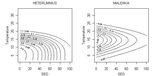Figure 8. Non-parametric relationship between probability of occurrence and temperature (°C) and percent sand/fines (SED) for Heterlimnius and Malenka. Contours represent mean probabilities of occurrence.

References

• Austin MP, Meyers JA (1996) Current approaches to modeling the environmental niche of eucalyptus: implication for management of forest biodiversity. Forest Ecology and Management 85:95-106.
• Hastie TJ, Tibshirani RJ (1999) Generalized Additive Models. Chapman & Hall/CRC, Washington DC.
• Oksanen J, Minchin PR (2002) Continuum theory revisited: what shape are species responses along ecological gradients. Ecological Modelling 157:119-129.

Top of Page