How RSIG Regrids Data
There are numerous approaches to regridding data each with varying complexity, performance and other trade-offs. RSIG regridding is optional, convenient, simple, and fast enough to be done on-the-fly during data subset retrieval.
- Summary of Regridding Options
- Regridding Occurs at the Source of the Data
- RSIG's Regridding Approach
- 2D/Swath Satellite Data Regridding
- 3D/Vertical Data Regridding
- Processing Time Limits
Summary of Regridding Options
RSIG regrids data by taking each data value and putting it into its own space/time grid. With each data value allocated in space and time, they are then aggregated.
- Spatial Allocation:
- Retrieval centroid in grid-cell
- Retrieval footprint overlap (for 2D satellite data with corners)
- Spatial Aggregation
- Simple mean
- Inverse distance weighted mean (for non 2D satellite data with corners)
- Fractional area overlap (for 2D satellite data with corners), with its own simple mean and weighted mean options
- Temporal Aggregation:
Regridding Occurs at the Source of the Data
The RSIG distributed software system includes data-specific Subset programs (e.g., MODISSubset) which read a set of data files and extract a subset of data into a single stream (in simple, efficient XDR format).
Another RSIG utility program, XDRConvert, is optionally invoked on the stream (pipe) to convert it to other formats (ASCII, NetCDF-coards, etc.) and also to optionally regrid/aggregate the data onto a (CMAQ) grid and streams that result.
Both the Subset program and XDRConvert are installed at the source of the data files (NASA Goddard for MODIS, NASA Langley for CALIPSO, etc.). This approach is efficient since regridded/aggregated results are usually much smaller so fewer bytes are streamed over the network.
RSIG's Regridding Approach
RSIG can optionally quickly regrid all data onto a structured, regular grid (in a projected space specified using M3IO (CMAQ) conventions).
Structured means the grid consists of a number of rows each with the same number of columns of cells.
Regular means all grid cells are the same shape/size.
In the projected space, such grids appear as a rectangle/square with rectangular/square cells.
This makes it simple and efficient to compute what grid cell a point projects into as shown in the C code below:
/*
 * Given:
 * arrays of point coordinates: longitudes[], latitudes[]
 * grid dimensions: [gridColumns, gridRows]
 * grid bounds: [gridXMinimum, gridXMaximum][gridYMinimum, gridYMaximum]
 * grid cell size: [cellWidth x cellHeight] and
 * pre-computed recipricols oneOverCellWidth, oneOverCellHeight
 */

#pragma omp parallel for reduction( + : griddedPointCount )

  for ( index = 0; index < count; ++index ) {
    const Real longitude = longitudes[ index ];
    const Real latitude  = latitudes[  index ];
    Real x = longitude;
    Real y = latitude;

    if ( projector ) { /* If grid is not in lon-lat space: */
      projector->project( projector, longitude, latitude, &x, &y );
    }

    if ( AND2( IN_RANGE( x, gridXMinimum, gridXMaximum ),
               IN_RANGE( y, gridYMinimum, gridYMaximum ) ) ) {
      const Real fractionalColumn = (x - gridXMinimum) * oneOverCellWidth  + 1.0;
      const Real fractionalRow    = (y - gridYMinimum) * oneOverCellHeight + 1.0;
      Integer column     = fractionalColumn; /* Truncate fraction. */
      Integer row        = fractionalRow;
      Real xCenterOffset = fractionalColumn - column - 0.5;
      Real yCenterOffset = fractionalRow    - row    - 0.5;
      xCenterOffset += xCenterOffset;
      yCenterOffset += yCenterOffset;

      if ( column > gridColumns ) {
        column = gridColumns;
        xCenterOffset = 1.0;
      }

      if ( row > gridRows ) {
        row = gridRows;
        yCenterOffset = 1.0;
      }

      CHECK4( IN_RANGE( column, 1, gridColumns ),
              IN_RANGE( row,    1, gridRows ),
              IN_RANGE( xCenterOffset, -1.0, 1.0 ),
              IN_RANGE( yCenterOffset, -1.0, 1.0 ) );

      /* ... Aggregate data value at into cell [column, row] ... */
      ++griddedPointCount;
    }
  }
- Projecting maps input (longitude, latitude) points into (x, y) projected space (e.g., Lambert Conformal Conic) of the grid. If the grid is defined in lon-lat space (e.g., 1/8-degree 2880 x 1440 global grid) then no projecting is required.
- During binning, each (possibly projected) data point is placed into a grid cell (or discarded if outside the grid).
- After binning is aggregation where the mean value in each grid cell is computed.
The grid's coordinate/projected space is defined by the various M3IO/CMAQ projection parameters described in the following table. All of the M3IO projectionsExitare supported, including lon-lat (e.g., 1/8-degree global grid). The most common is Lambert Conformal Conic used over CONUS:
| Parameter | Description |
|---|---|
| P_ALP = 33 | Lower latitude of secant of plane intersecting the globe |
| P_BET = 45 | Upper latitude of secant of plane intersecting the globe |
| XCENT (=P_GAM) = -97 | Center longitude that projects to 0 |
| YCENT = 40 | Latitude that projects to 0 |
| Mean Earth Radius = 6,370,000 (m) | User-specified value (from configuration scripts when they ran the CMAQ (and MET) models). |
In this projected space, the CMAQ grid is regular and defined by the following parameters:
| Parameter | Description |
|---|---|
| NCOLS = 268 | Number of columns of grid cells |
| NROWS = 259 | Number of rows of grid cells |
| XORIG = -420000 (m) | Horizontal distance, in meters, from the lower-left corner of the grid to the projection origin (-97,40) |
| YORIG = -1716000 (m) | Vertical distance, in meters, from the lower-left corner of the grid to the projection origin (-97,40) |
| XCELL = 12000 (m) | Width, in meters, of each grid cell |
| YCELL = 12000 (m) | Height, in meters, of each grid cell |
Each data point to be regridded has (longitude, latitude) coordinates which are projected into (x, y) meters. Projecting involves computing various trigonometric formulas, some of which are derived from projection parameters and thus pre-computed for efficiency. For reference, see PROJ Library Exit(not used by RSIG).)
Points that are outside the grid are discarded. Cells that receive no data points are given the value -9.999E+36 (BADVAL3). Cells that receive more than one data value are aggregated using one of two user-specified methods, explained in the following table:
| Method | Description |
|---|---|
| REGRID=mean | The mean of all values within the cell is used. I.e., the values are summed and counted and, at the end, the sum is divided by the count to obtain the mean. |
| REGRID=weighted | The inverse-distance-weighted (1/r2) mean is used. I.e., the values are weighted (multiplied) by the square of the inverse distance to the cell center and summed and the weights are summed. At the end, the cell value is divided by the weight sum to obtain the weighted mean. For 2D/swath satellite data, area-weighting is used as described in the next section. |

Figure 1: Illustration of RSIG's project/aggregation process with a simplified CMAQ grid of only 3x2 (large) cells over the Western US.
The following table describes the aggregation timestep size, which can be user-specified.
No temporal-distance weighting is done as most data in RSIG is already GMT hourly and sub-hourly data, such as from polar-orbiting satellites, have 5-minute timestamps that move outside the grid on the next timestep.
Results can be saved in various formats such as ASCII, XDR, and NetCDF-COARDS. These formats never include "missing/invalid" data values, which are filtered out during the subsetting process. The exception is NetCDF-IOAPI -- such files must contain complete/structured grids and tend to be much larger (100x) than the other formats.
Choosing FORMAT=netcdf-ioapi results in a time-aggregated single layer CMAQ grid file for each regridded data source. This is compatible with existing programs that can read CMAQ files (e.g., PAVEExit, VERDIExit). Note that most grid cells will contain the value -9.999E+36 (BADVAL3) to indicate "missing" since the other data is relatively spatially and temporally sparse compared to the CMAQ grid.
RSIG does not implement methods to "fill-in-the-empty-cells" (e.g., krigingExit). If users want to generate such data, they can do so starting from either the regridded data output from RSIG or the unregridded RSIG-subsetted data (e.g., FORMAT=netcdf-coards).
2D/Swath Satellite Data Regridding
From Points to Quadrilaterals: CORNERS=1 Option
Level-2 satellite data such as MODIS, VIIRS, TROPOMI, etc. consist of a number of rows and columns of data points arranged into a swath/granule (warped patch) on the Earth surface.
At nadir (when the satellite instrument is pointing straight down to the Earth's surface these points are close together (10km for MODIS MOD04-L2, 750m for VIIRS, etc.) and when the instrument is scanning to the sides, these points are spaced further apart (40km for MODIS, etc.). This results in a warped patch of points. However, each point actually represents the center of a small area on the Earth surface where the averaged measurement occurs over a short time period.
These points, often referred to as pixels, are more like polygons that may overlap slightly with neighboring polygons and have gaps between neighboring polygons.
In RSIG, these small areas are represented simply as quadrilaterals whose corner vertices (geometric dual) are easily computed by linearly interpolating the surrounding center points (simply averaging the neighboring coordinates) and extrapolating to the edges.
This computation is done when specifying the option CORNERS=1 (always done in RSIG3D) and results in a 2D curvilinear grid of non-overlapping, connected (non-gapped) quadrilaterals -- except that satellite data points may be missing/filtered-out so their quadrilaterals will also be omitted.
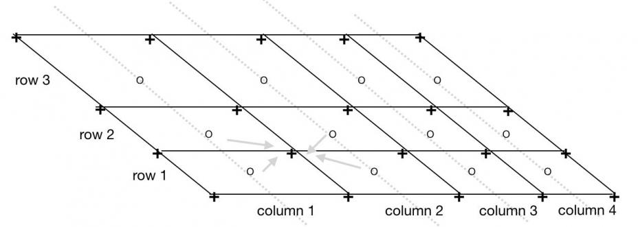
Figure 2: Computing corner vertices from satellite swath center points.
- o = input 3 rows of 4 columns of swatch center points on instrument scan lines
- + = output quadrilaterial corner vertices (lon,lat)
- Each corner vertex has (lon,lat) coordinates that are the average of the coordinates of the surrounding center points. E.g.,
corner _longitude[row][column][SW] = 0.25 * (center_lon[row][column] + center_lon[row-1 ][column] + center_lon[row-1 ][column-1] + center_lon[row][column-1]). - Edge corners are linearly extrapolated from the neighboring interior corners.
This method yields a curvilinear grid of gap-free non-overlapping quadrilaterals suitable for fast rendering and regridding.
From Quadrilaterals to Grid Cells
When binning these 2D quadrilaterals, their corner vertices are projected (as described above) resulting in quadrilaterals (in projected space) landing in 0, 1 or several adjacent grid cells.
That is, depending on the relative size of the grid cells to the satellite data quadrilaterals, a quadrilateral may land entirely outside the grid (and be discarded) or entirely inside a single grid cell (easy, just use weight = 1) or spread across several adjacent grid cells.
In this latter case, extra computation will occur, depending on the REGRID option:
The REGRID=weighted option requires clipping a satellite data convex quadrilateral to each intersecting grid cell rectangle which yields one polygon per intersecting grid cell.
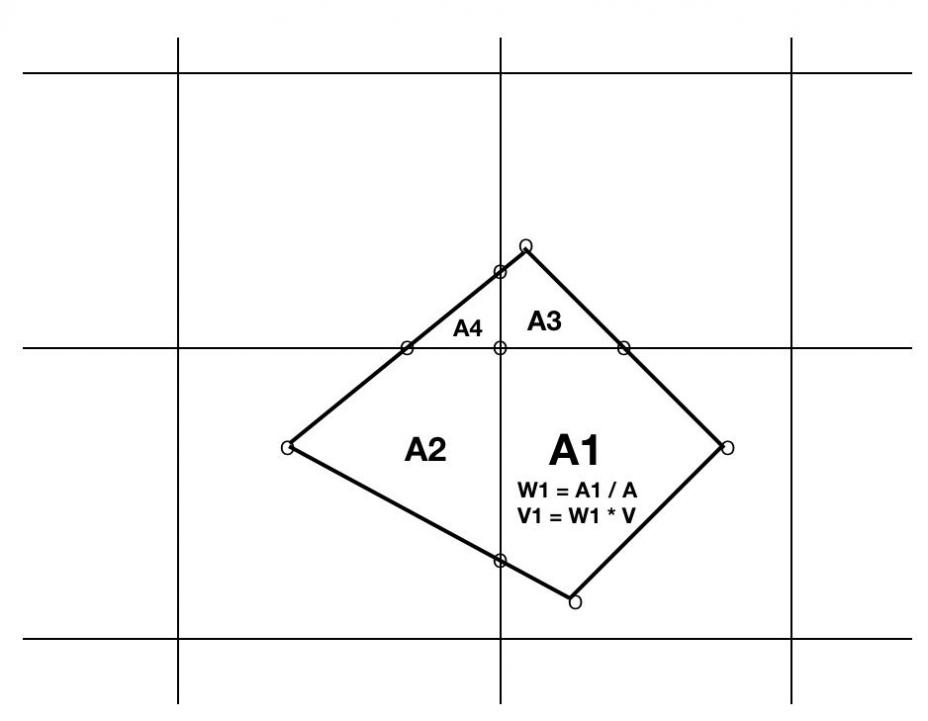
Figure 3: Binning a satellite datum quadrilateral into 4 intersecting grid cells.
- V = value of satellite measurement for quadrilateral
- A= area of entire quadrilateral
- Ai= area of ith polygon fragment of quadrilateral clipped to ith grid cell
- Wi = weight of ith portion = Ai / A summed into ith grid cell
- Vi = fraction of datum summed into ith grid cell = Wi * V
- Final mean aggregate of value in ith grid cell = sum(Vi)/sum(Wi)
While non-trivial, RSIG uses the fastest-known polygon clipping algorithm (Liang-Barsky, CACM Nov. 1983Exit) (and 1,000 lines of optimized stand-alone code spread over more than a dozen routines) to yield fast, on-the-fly regridding. The C polygon clipping and area calculation routines are shown below.
/******************************************************************************
PURPOSE: clipPolygon - Clip polygon to an axis-aligned rectangle
         and return the number of vertices in clipped polygon.
INPUTS:  const int discardDegenerates  Discard degenerate triangles?
                                       Slower, but useful if rendering.
         const double clipXMin  X-coordinate of lower-left  corner of clip rect
         const double clipYMin  Y-coordinate of lower-left  corner of clip rect
         const double clipXMax  X-coordinate of upper-right corner of clip rect
         const double clipYMax  Y-coordinate of upper-right corner of clip rect
         const int count          Number of input vertices.
         const double x[ count ]  X-coordinates of input polygon to clip.
         const double y[ count ]  Y-coordinates of input polygon to clip.
         double cx[ 2 * count + 2 ]  Storage for 2 * count + 2 X-coordinates.
         double cy[ 2 * count + 2 ]  Storage for 2 * count + 2 Y-coordinates.
OUTPUTS: double cx[ result ]      X-coordinates of vertices of clipped poly.
         double cy[ result ]      Y-coordinates of vertices of clipped poly.
RETURNS: int number of vertices in clipped polygon.
NOTES:   Uses the Liang-Barsky polygon clipping algorithm. (Fastest known.)
         "An Analysis and Algorithm for Polygon Clipping",
         You-Dong Liang and Brian Barsky, UC Berkeley,
         CACM Vol 26 No. 11, November 1983.
         https://www.longsteve.com/fixmybugs/?page_id=210
******************************************************************************/

static int clipPolygon( const int discardDegenerates,
                        const double clipXMin,
                        const double clipYMin,
                        const double clipXMax,
                        const double clipYMax,
                        const int count,
                        const double x[],
                        const double y[],
                        double cx[],
                        double cy[] ) {
  int result = 0;
  const double inf = DBL_MAX;
  double xIn   = 0.0; /* X-coordinate of entry point. */
  double yIn   = 0.0; /* Y-coordinate of entry point. */
  double xOut  = 0.0; /* X-coordinate of exit point. */
  double yOut  = 0.0; /* Y-coordinate of exit point. */
  double tInX  = 0.0; /* Parameterized X-coordinate of entry intersection. */
  double tInY  = 0.0; /* Parameterized Y-coordinate of entry intersection. */
  double tOutX = 0.0; /* Parameterized X-coordinate of exit intersection. */
  double tOutY = 0.0; /* Parameterized Y-coordinate of exit intersection. */
  int vertex = 0;

  for ( vertex = 0; vertex < count; ++vertex ) {
    const int vertexp1 = vertex + 1;
    const int vertex1 = vertexp1 < count ? vertexp1 : 0;
    const double vx = x[ vertex ];
    const double vy = y[ vertex ];
    const double deltaX = x[ vertex1 ] - vx; /* Edge direction. */
    const double deltaY = y[ vertex1 ] - vy;
    const double oneOverDeltaX = deltaX ? 1.0 / deltaX : 0.0;
    const double oneOverDeltaY = deltaY ? 1.0 / deltaY : 0.0;
    double tOut1 = 0.0;
    double tOut2 = 0.0;
    double tIn2 = 0.0;
    assert( result < count + count + 2 );

    /*
     * Determine which bounding lines for the clip window the containing line
     * hits first:
     */

    if ( deltaX > 0.0 || ( deltaX == 0.0 && vx > clipXMax ) ) {
      xIn  = clipXMin;
      xOut = clipXMax;
    } else {
      xIn  = clipXMax;
      xOut = clipXMin;
    }

    if ( deltaY > 0.0 || ( deltaY == 0.0 && vy > clipYMax ) ) {
      yIn  = clipYMin;
      yOut = clipYMax;
    } else {
      yIn  = clipYMax;
      yOut = clipYMin;
    }

    /* Find the t values for the x and y exit points: */

    if ( deltaX != 0.0 ) {
      tOutX = ( xOut - vx ) * oneOverDeltaX;
    } else if ( vx <= clipXMax && clipXMin <= vx ) {
      tOutX = inf;
    } else {
      tOutX = -inf;
    }

    if ( deltaY != 0.0 ) {
      tOutY = ( yOut - vy ) * oneOverDeltaY;
    } else if ( vy <= clipYMax && clipYMin <= vy ) {
      tOutY = inf;
    } else {
      tOutY = -inf;
    }

    /* Set tOut1 = min( tOutX, tOutY ) and tOut2 = max( tOutX, tOutY ): */

    if ( tOutX < tOutY ) {
      tOut1 = tOutX;
      tOut2 = tOutY;
    } else {
      tOut1 = tOutY;
      tOut2 = tOutX;
    }

    if ( tOut2 > 0.0 ) {

      if ( deltaX != 0.0 ) {
        tInX = ( xIn - vx ) * oneOverDeltaX;
      } else {
        tInX = -inf;
      }

      if ( deltaY != 0.0 ) {
        tInY = ( yIn - vy ) * oneOverDeltaY;
      } else {
        tInY = -inf;
      }

      /* Set tIn2 = max( tInX, tInY ): */

      if ( tInX < tInY ) {
        tIn2 = tInY;
      } else {
        tIn2 = tInX;
      }

      if ( tOut1 < tIn2 ) { /* No visible segment. */

        if ( 0.0 < tOut1 && tOut1 <= 1.0 ) {
          assert( result < count + count );

          /* Line crosses over intermediate corner region. */

          if ( tInX < tInY ) {
            cx[ result ] = xOut;
            cy[ result ] = yIn;
          } else {
            cx[ result ] = xIn;
            cy[ result ] = yOut;
          }

          ++result;
        }
      } else { /* Line crosses through window: */

        if ( 0.0 < tOut1 && tIn2 <= 1.0 ) {

          if ( 0.0 <= tIn2 ) { /* Visible segment: */
            assert( result < count + count );

            if ( tInX > tInY ) {
              cx[ result ] = xIn;
              cy[ result ] = vy + ( tInX * deltaY );
            } else {
              cx[ result ] = vx + ( tInY * deltaX );
              cy[ result ] = yIn;
            }

            ++result;
          }

          assert( result < count + count );

          if ( 1.0 >= tOut1 ) {

            if ( tOutX < tOutY ) {
              cx[ result ] = xOut;
              cy[ result ] = vy + ( tOutX * deltaY );
            } else {
              cx[ result ] = vx + ( tOutY * deltaX );
              cy[ result ] = yOut;
            }

            ++result;
          } else {
            cx[ result ] = x[ vertex1 ];
            cy[ result ] = y[ vertex1 ];
            ++result;
          }
        }
      }

      if ( 0.0 < tOut2 && tOut2 <= 1.0 ) {
        assert( result < count + count );
        cx[ result ] = xOut;
        cy[ result ] = yOut;
        ++result;
      }
    }
  }

  /*
   * The above algorithm can generate 5-vertex 'line' or 'hat' polygons: _/\_
   * where the last 3 vertices are colinear
   * which yields a degenerate 'triangle' (i.e., with 0 area).
   * Here we discard the last 2 verticies in such cases.
   */

  if ( discardDegenerates && result == 5 ) {
    int twice = 2; /* Check twice in case of 5-vertex 'line'. */

    do {

      if ( result >= 3 ) {
        const size_t count_3 = result - 3;
        const size_t count_2 = result - 2;
        const size_t count_1 = result - 1;

        const double lastTriangleArea =
          areaOfTriangle( cx[ count_3 ], cy[ count_3 ],
                          cx[ count_2 ], cy[ count_2 ],
                          cx[ count_1 ], cy[ count_1 ] );

        if ( lastTriangleArea == 0.0 ) {
          result -= 2;
        }
      }
    } while ( --twice );
  }

  /* Always discard any result less than a triangle. */

  if ( result < 3 ) {
    result = 0;
  }

  assert( result == 0 || IN_RANGE( result, 3, count + count + 2 ) );
  return result;
}


/******************************************************************************
PURPOSE: areaOfTriangle - Absolute/unsigned area of triangle with vertices
         (x1, y1), (x2, y2), (x3, y3).
INPUTS:  const double x1  X-Coordinate of 1st vertex of triangle.
         const double y1  Y-Coordinate of 1st vertex of triangle.
         const double x2  X-Coordinate of 2nd vertex of triangle.
         const double y2  Y-Coordinate of 2nd vertex of triangle.
         const double x3  X-Coordinate of 3rd vertex of triangle.
         const double y3  Y-Coordinate of 3rd vertex of triangle.
RETURNS: double area.
NOTES:   Area = 0.5 * |p X q|
         Where p and q are vectors of the triangle:
         p being from 1st vertex to 2nd vertex and
         q being from 1st vertex to 3rd vertex.
         and X is the 2D vector cross-product binary operator:
         p X q = px * qy - qx * py.
         http://geomalgorithms.com/a01-_area.html
******************************************************************************/

static double areaOfTriangle( const double x1, const double y1,
                              const double x2, const double y2,
                              const double x3, const double y3 ) {
  const double px = x2 - x1;
  const double py = y2 - y1;
  const double qx = x3 - x1;
  const double qy = y3 - y1;
  const double cross = px * qy - qx * py;
  const double abscross = cross < 0.0 ? -cross : cross;
  const double result = 0.5 * abscross;
  assert( result >= 0.0 );
  return result;
}


/******************************************************************************
PURPOSE: areaOfQuadrilateral - Absolute/unsigned area of quadrilateral with
         vertices (x1, y1), (x2, y2), (x3, y3), (x4, y4).
INPUTS:  const double x1  X-Coordinate of 1st vertex of quadrilateral.
         const double y1  Y-Coordinate of 1st vertex of quadrilateral.
         const double x2  X-Coordinate of 2nd vertex of quadrilateral.
         const double y2  Y-Coordinate of 2nd vertex of quadrilateral.
         const double x3  X-Coordinate of 3rd vertex of quadrilateral.
         const double y3  Y-Coordinate of 3rd vertex of quadrilateral.
         const double x4  X-Coordinate of 4th vertex of quadrilateral.
         const double y4  Y-Coordinate of 4th vertex of quadrilateral.
RETURNS: double area.
NOTES:   Area = 0.5 * |p X q|
         Where p and q are diagonal vectors of the quadrilateral:
         p being from 1st vertex to 3rd vertex and
         q being from 4th vertex to 2nd vertex.
         and X is the 2D vector cross-product binary operator:
         p X q = px * qy - qx * py.
         http://mathworld.wolfram.com/Quadrilateral.html
         http://mathworld.wolfram.com/CrossProduct.html
******************************************************************************/

static double areaOfQuadrilateral( const double x1, const double y1,
                                   const double x2, const double y2,
                                   const double x3, const double y3,
                                   const double x4, const double y4 ) {
  const double px = x3 - x1;
  const double py = y3 - y1;
  const double qx = x2 - x4;
  const double qy = y2 - y4;
  const double cross = px * qy - qx * py;
  const double abscross = cross < 0.0 ? -cross : cross;
  const double result = 0.5 * abscross;
  assert( result >= 0.0 );
  return result;
}


/******************************************************************************
PURPOSE: signedAreaOfPolygon - Signed area of a single contour of a polygon.
INPUTS:  const size_t count  Number of vertices in polygon.
         const double x[]    X-coordinates of vertices.
         const double y[]    Y-coordinates of vertices.
RETURNS: double signed area of polygon.
         Negative if vertices are in clockwise order.
NOTES:   http://mathworld.wolfram.com/PolygonArea.html
******************************************************************************/

static double signedAreaOfPolygon( const size_t count,
                                   const double x[], const double y[] ) {
  double result = 0.0;
  size_t index = 0;

  for ( index = 0; index < count; ++index ) {
    const size_t indexp1 = index + 1;
    const size_t index1 = indexp1 < count ? indexp1 : 0;
    const double triangleArea =
      x[ index ] * y[ index1 ] - x[ index1 ] * y[ index ];
    result += triangleArea;
  }

  result *= 0.5;
  return result;
}
3D/Vertical Data Regridding
CALIPSO LIDAR provides 3D data that exists as a column of points from the surface up to 40km high. Other data sources such as NEUBrew spectrophotometers, ceilometers, and MOZAIC aircraft also yield points with elevations above the surface.
These points are regridded into the CMAQ layers by using the CMAQ vertical grid description parameters NLAYS, VGTOP, VGLVLS (sigma pressures), etc. to compute the CMAQ levels in meters above mean sea level and aggregate multiple points within a single CMAQ grid cell (using the same scheme: mean, distance-weighted mean).
Vertical regridding occurs when including the vertical CMAQ grid parameters LEVELS= in the WCS request to rsigserver, e.g.,
REGRID=weighted&LAMBERT=33,45,-97,40&ELLIPSOID=6370997,6370997&
GRID=268,259,-420000,-1716000,12000,12000&
LEVELS=22,2,10000,1.0,0.995,0.988,0.979,0.97,0.96,0.938,0.914,0.889,0.862,
0.834,0.804,0.774,0.743,0.694,0.644,0.592,0.502,0.408,0.311,0.21,0.106,0.0,
9.81,287.04,50,290,100000
The regridding computation occurs at the remote source of the data (e.g., NASA Goddard server running RSIG XDRConvert program) and only the regridded (usually greatly reduced) data is streamed back.
Since the formulas that relate sigma-pressures to meters (see routine below) require the surface elevation, the surface elevation used is that measured by the CALIPSO satellite which can differ slightly from the averaged (e.g., 12km) terrain height of the CMAQ grid cell.
Following is the C routine that computes the elevation in meters above mean sea level from the CMAQ sigma-pressure levels.
/******************************************************************************
PURPOSE: elevationsAtSigmaPressures - Compute elevations in meters above mean
         sea-level at sigma-pressures.
INPUTS:  Real g                Gravitational force, e.g., 9.81 m/s^2.
         Real R                Gas constant e.g., 287.04 J/kg/K = m^3/s/K.
         Real A                Atmospheric lapse rate, e.g., 50.0 K/kg.
         Real T0s              Reference surface temperature, e.g., 290.0 K.
         Real P00              Reference surface pressure, e.g., 100000 P.
         Real surfaceElevation     Elevation of surface in meters AMSL.
         Integer levels            Number of levels of sigmaPressures.
         Real topPressure          Pressure in Pascals at the top of the model.
         const Real sigmaPressures[ levels ]  Sigma-pressures at levels.
OUTPUTS: Real elevations[ levels ]  Elevation in meters above MSL at sigmas.
NOTES:   Based on formula used in MM5.
******************************************************************************/

static void elevationsAtSigmaPressures( Real g, Real R, Real A, Real T0s,
                                        Real P00,
                                        Real surfaceElevation,
                                        Integer levels, Real topPressure,
                                        const Real sigmaPressures[],
                                        Real elevations[] ) {

  PRE014( ! isNan( g ),
          ! isNan( R ),
          ! isNan( A ),
          ! isNan( T0s ),
          ! isNan( P00 ),
          ! isNan( surfaceElevation ),
          surfaceElevation > -1000.0,
          levels > 0,
          ! isNan( topPressure ),
          GT_ZERO6( topPressure, g, R, A, T0s, P00 ),
          isNanFree( sigmaPressures, levels ),
          minimumItem( sigmaPressures, levels ) >= 0.0,
          maximumItem( sigmaPressures, levels ) <= 1.0,
          elevations );

  /* Derived constants: */

  const Real H0s            = R * T0s / g;
  const Real one_over_H0s   = 1.0 / H0s;
  const Real A_over_T0s     = A / T0s;
  const Real A_over_two_T0s = A / ( T0s + T0s );
  const Real Pt             = topPressure;
  const Real Zs             = surfaceElevation;
  const Real two_Zs         = Zs + Zs;
  const Real sqrt_factor    = sqrt( 1.0 - A_over_T0s * one_over_H0s * two_Zs );
  const Real q_factor =
   ( Pt / P00 ) * exp( two_Zs * one_over_H0s / sqrt_factor );
  Integer level = 0;

  /* Compute elevations at sigma-pressures: */

  for ( level = 0; level < levels; ++level ) {
    const Real sigma_p0   = sigmaPressures[ level ];
    const Real q0_star    = sigma_p0 + ( 1.0 - sigma_p0 ) * q_factor;
    const Real ln_q0_star = log( q0_star );
    const Real z_level    =
      Zs - H0s * ln_q0_star * ( A_over_two_T0s * ln_q0_star + sqrt_factor );
    elevations[ level ]   = z_level;
  }

  POST03( isNanFree( elevations, levels ),
          minimumItem( elevations, levels ) >= -1000.0,
          maximumItem( elevations, levels ) <= 1e6 );

}
Here are some computed level elevations compared to the values in the MET files:
level   West-formula  West ZF ocean     East-formula   East ZF ocean
--------------------------------------------------------------------
0          -0.0           0.0            -0.0            0.0
1          36.3          36.3            38.3           38.3
2          72.7          72.7            76.7           76.7
3         145.9         146.0           153.9          154.0
4         294.0         294.2           310.1          310.9
5         444.4         444.7           468.8          469.0
6         674.5         674.8           711.5          711.9
7        1070.4        1070.9          1129.5         1130.1
8        1568.0        1568.8          1655.1         1656.0
9        2093.0        2094.1          2210.0         2211.1
10       2939.6        2941.1          3105.6         3107.2
11       3980.5        3982.5          4208.4         4210.5
12       5807.2        5810.2          6148.1         6151.2
13       9057.5        9062.2          9616.2         9621.2
14      14649.4       14656.8         15660.0        15668.0
Regridding Examples
# 24-hours of TROPOMI NO2 over CONUS (takes about 30 seconds and yields 52MB):

curl -k --silent --retry 0 -L --tcp-nodelay --max-time 0  \
'http://ofmpub.epa.gov/rsig/rsigserver?SERVICE=wcs&VERSION=1.0.0&REQUEST=GetCoverage&
COVERAGE=tropomi.offl.no2.nitrogendioxide_tropospheric_column&minimum_quality=75&
TIME=2020-10-01T00:00:00Z/2020-10-01T23:59:59Z&
BBOX=-136,20,-53,57&
CORNERS=1&
REGRID=weighted&LAMBERT=33,45,-97,40&ELLIPSOID=6370000,6370000&
GRID=459,299,-2556000,-1728000,12000,12000&
COMPRESS=0&FORMAT=netcdf-ioapi'  > regridded_tropomi_no2_hourly.ncf

# 7 days of TROPOMI NO2 over CONUS (takes about 3 minutes and yields 15MB):

curl -k --silent --retry 0 -L --tcp-nodelay --max-time 0  \
'http://ofmpub.epa.gov/rsig/rsigserver?SERVICE=wcs&VERSION=1.0.0&REQUEST=GetCoverage&
COVERAGE=tropomi.offl.no2.nitrogendioxide_tropospheric_column&minimum_quality=75&
TIME=2020-10-01T00:00:00Z/2020-10-07T23:59:59Z&
BBOX=-136,20,-53,57&
CORNERS=1&
REGRID=weighted&LAMBERT=33,45,-97,40&ELLIPSOID=6370000,6370000&
GRID=459,299,-2556000,-1728000,12000,12000&
REGRID_AGGREGATE=daily&
COMPRESS=0&FORMAT=netcdf-ioapi'  > regridded_tropomi_no2_daily.ncf

# 1 week average of TROPOMI NO2 over CONUS (takes about 3 minutes and yields 2MB):

curl -k --silent --retry 0 -L --tcp-nodelay --max-time 0  \
'http://ofmpub.epa.gov/rsig/rsigserver?SERVICE=wcs&VERSION=1.0.0&REQUEST=GetCoverage&
COVERAGE=tropomi.offl.no2.nitrogendioxide_tropospheric_column&minimum_quality=75&
TIME=2020-10-01T00:00:00Z/2020-10-07T23:59:59Z&
BBOX=-136,20,-53,57&
CORNERS=1&
REGRID=weighted&LAMBERT=33,45,-97,40&ELLIPSOID=6370000,6370000&
GRID=459,299,-2556000,-1728000,12000,12000&
REGRID_AGGREGATE=all&
COMPRESS=0&FORMAT=netcdf-ioapi'  > regridded_tropomi_no2_week.ncf
Processing Time Limits
Requests for large amounts of data processing -- e.g., months or years of data, whether regridding or not -- may fail due to http timeout after 30 minutes before completion.
Note most of the time for processing is not the regridding phase but rather the reading of the many input data files. For example, typical satellite data files are produced every 5 minutes so a request to process a month of files involves reading (a subset of data from) thousands of files. This time for file reading (by the data-specific Subset program) far outweighs the time to compute regridding (by XDRConvert). If you need to process/regrid large amounts of data (months or years of data) the RSIG Staff can create and run scripts to do this quickly and deliver the resulting files to you via ftp.