ten Berge Concentration x Time Model (Use with Benchmark Dose Software (BMDS) v2.7)
The ten Berge model has been superseded by EPA’s categorical regression software CatReg.
BMDS 2.7 is no longer under active development. With a few exceptions, most models are now maintained in BMDS 3.x.
The ten Berge Concentration × Time (C × T) Model is a unique model within BMDS, as it allows for more than one explanatory variable in a dichotomous dataset to influence response![]() responseThe biological result of an exposure or dose. Biological responses can be quantified in several ways. Some examples of the type of response data that can be used in a BMD dose-response analysis are dichotomous data (quantal data), nested data, continuous data, and categorical data. (for example, dose and time). C × T modeling is primarily used in the context of acute inhalation exposures, and is based on Haber’s Law (C × T = k).
responseThe biological result of an exposure or dose. Biological responses can be quantified in several ways. Some examples of the type of response data that can be used in a BMD dose-response analysis are dichotomous data (quantal data), nested data, continuous data, and categorical data. (for example, dose and time). C × T modeling is primarily used in the context of acute inhalation exposures, and is based on Haber’s Law (C × T = k).
Haber’s Law assumes a consistency across chemicals (i.e., a linear relationship between exposure concentration and duration) that may not be true for predicting response for all chemicals. The ten Berge model does not assume a linear relationship as it includes an exponent term on the C parameter (i.e., the conceptual model form is Cn × T = k). When n >1, the response is considered concentration-dependent (i.e., response is more influenced by increases/decreases in exposure concentration); when n <1, the response is time-dependent.
Note: The ten Berge model can only be run from BMDS. You cannot use the BMDS Wizard to run the ten Berge model.
For more conceptual information on the ten Berge C × T model, refer to the ten Berge model documentation. For information on BMDS's ten Berge implementation, refer to the BMDS Help file or the BMDS User Manual (located in the BMDS application folder).
- Before You Start
- Exercise
- ten Berge Text Results
- ten Berge Graph Results
- Estimation of Ratio Between Regression Coefficients
Before You Start
Download tenberge_exercise.zip (ZIP)(1 pg, 498 B) and extract the tenberge_qs.dax file to the BMDS Data subdirectory on your computer. You will use this dataset for the following exercise.
Exercise
- The ten Berge model can only be run from BMDS. In BMDS, select File>Open>Dataset (.dax). In the Open dialog box, select the tenBerge_qs.dax file and click Open. BMDS displays the dataset in a new Data Grid window.
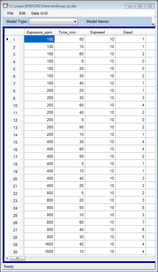
- Data presented in sequential columns (i.e., column 1 = dose, column 2 = time, etc.).
- The first columns in the dataset should be the Main Effect columns (e.g., Dose and Time). These columns can be in any order but they must appear first.
- The final columns in the dataset should be the # Subjects and Incidence columns, in that order.
- Other columns (e.g., Age, Litter) can appear in any order following the Main Effect columns but before the # Subjects and Incidence.
- Minimum data requirements: the total number of subjects, the number of affected subjects, and two explanatory variables.
- In the Data Grid window, from the Model Type picklist, select Conc_x_Time. BMDS automatically populates the Model Name field with ten Berge. Click the Proceed button to display the Model Options screen for ten Berge.
- Make sure your Model Options screen matches the following screenshot:
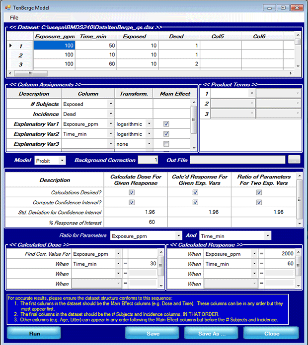
- The value for one explanatory variable given a response level of interest and the value for the other explanatory variable,
- The response level given values for both explanatory variables, and
- The ratio of regression coefficients for the explanatory variables (i.e., the value of n when concentration and time are used).
- Click Run to run the model. BMDS displays the C × T results in an .out file and exports them to an Excel template file containing two customizable plots.
The remainder of this exercise will describe the .out files and the Excel plots.
ten Berge Text Results
- Estimation of Exposure_ppm
- Estimation of response
- Estimation of ratio between regression coefficients
Estimation of Exposure_ppm
Estimation of Exposure_ppm
Response = 60.000000 percent
Time_min = 30.000000
Estimated Exposure_ppm 60.000000 percent = 1.650e+003
Deviate Corresponding to Confidence Level of Interest = 1.960000
Lower limit Exposure_ppm 60.000000 percent = 1.240e+003
Upper limit Exposure_ppm 60.000000 percent = 2.417e+003
Probability of correct model (p-value) is 0.954560
The prediction of the model is sufficient. Use for estimation of the
95% confidence limits the Standard Normal Deviate
No correction for variances required!
Estimation of response
Estimation of response
Exposure_ppm = 2000.000000
Time_min = 60.000000
Response = 7.55e+001 percent
Deviate Corresponding to Confidence Level of Interest = 1.960000
LL-response = 6.69e+001 percent
UL-response = 8.27e+001 percent
Probability of correct model (p-value) is 0.954560
The prediction of the model is sufficient. Use for estimation of the
95% confidence limits the Standard Normal Deviate
No correction for variances required!
Estimation of ratio between regression coefficients
Estimation of ratio between regression coefficients
Ratio between regression coefficients
Exposure_ppm and Time_min
Deviate Corresponding to Confidence Level of Interest = 1.960000
Ratio = 1.154502
Confidence limits
0.699105 1.609898
ten Berge Graph Results
BMDS creates the plots using the following Excel file (assuming a standard BMDS installation): \<BMDS Program Directory>\SysData\tenBergePlotTemplate.xls. You may want to save this file to a different name or path if you want to work with the results later.
Contour of Constant Probability
The constant probability plot shows the contour of concentration and time combinations for a user-specified probability. It corresponds to the Estimation of Exposure_ppm result.
The .out file's Estimated Exposure_ppm for a 60% response of interest at 30 minutes is 1.650e+003 (e.g., 1650 ppm). We want the constant probability contour graph to show what combination of time (x-axis) and concentration (y-axis) results in a 60% response.
To do that, you may need to edit the following cell in the spreadsheet to generate the plot:
- In cell E23, enter .6 (corresponding to the 60% response). The plot should redraw accordingly.
Leave cells E25, E26, and E27 unchanged. We did not specify 3rd, 4th, or 5th explanatory variables on the BMDS Options screen.
On the contour plot, hover the pointer at or as close to 30 minutes as you can along the x-axis. Excel should display the values “30, 1.65E+003” at that point. (You may need to zoom in on the graph to find the exact point.)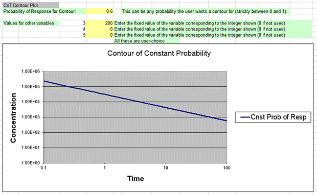
Probability of Response
The probability of response plot is a function of either concentration or time. It corresponds to the .out file's Estimation of response result.
The .out file's Estimation of response for an exposure of 2000ppm for 60 minutes is 75.5%.
To generate a “traditional” dose-response curve (i.e., a plot of where the independent variable (x-axis) is dose and the dependent variable (y-axis) is response), you need to edit the following cells in the spreadsheet:
- The maximum values for var1 and var2 should come from the tenberge_qs.dax dataset.
- In cell C60, enter 3200 as the maximum value for var1 (Concentration).
- In cell C63, enter 60 as the maximum value for var2 (Time).
- In cell E68, enter 60 for var2, corresponding to "60 minutes" as the specific value for the fixed variable.
- Cells E69, E70, and E71 should contain "0" because we are not specifying 3rd, 4th, or 5th explanatory variables.
Editing the plot's numbers as above will result in a dose-response curve plotting response (y-axis) against dose (x-axis) for an exposure lasting 60 minutes.
You should get a graph that looks like the following screenshot. Hover the mouse pointer along the curve until it intersects at 2000 along the x-axis; Excel should display the values at that point as “2000, 0.754848794.”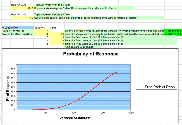
You can also generate a plot where the independent variable (x-axis) is time. To do this, edit the spreadsheet cells for the plot as follows:
- The maximum values for var1 and var2 should come from the tenberge_qs.dax file.
- In cell C60, enter 3200 as the maximum value for var1 (Concentration).
- In cell C63, enter 60 as the maximum value for var2 (Time).
- In cell D67, enter 2 as the Variable #
- In cell D68, enter 1 as the Variable #
- In cell E68, enter 2000 for var1, corresponding to "2000 ppm" as the specific value for the fixed variable.
- Leave cells E69, E70, and E71 at "0" because we are not specifying 3rd, 4th,or 5th explanatory variables.
Editing the plot's numbers as above will result in a dose-response curve plotting response (y-axis) against time (x-axis) for an exposure of 2000 ppm.
You should get a graph that looks like the following screenshot (you will need to manually edit the plot's horizontal axis using Excel's Format Axis command to show the minimum bound as 1.0 and the maximum bound as 100.0). Hover the mouse pointer along the curve until it intersects at 60 along the x-axis; Excel should display the values at that point as “60, 0.754848794.”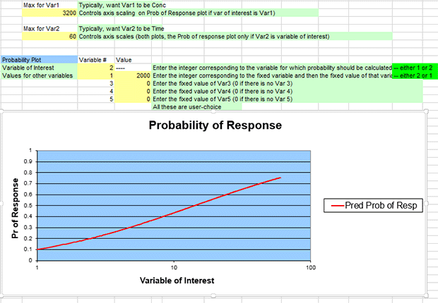
Estimation of Ratio Between Regression Coefficients
In this example, the ten Berge model was run with exposure concentration (variable 1) and time (variable 2) logarithmically transformed.
Therefore, the ratio between the regression coefficients (b1 and b2) for these two parameters gives the value of n in the equation Cn × T = k. In this example, as we see from the .out file results, n = 1.154502. We also see that the 95% confidence interval on this value is (0.699105, 1.609898). In this example, because the confidence level is nonsignificant, the response is potentially concentration dependent. Or, put another way: increases/decreases in exposure concentration influence the responses to a potentially greater degree than do changes in the duration of exposure. However, if the duration of exposure was more significant than the exposure concentration, then we would expect to see values of n less than 1.
