Urbanization - Hydrology
Flow Alteration in Urban Streams
Alteration of natural hydrologic regimes is a consistent and pervasive effect of urbanization on stream ecosystems. Discharge patterns—the amount and timing of water flow through streams—change with urban development. Key aspects of urbanization affecting hydrology may include:
- Decreased infiltration and increased surface runoff of precipitation associated with impervious (and effectively impervious) surfaces
- Increased speed and efficiency of runoff delivery to streams, via stormwater drainage infrastructure
- Decreased evapotranspiration due to vegetation removal
- Increased direct water discharges, via wastewater and industrial effluents
- Increased infiltration due to irrigation and leakage from water supply and wastewater infrastructure
- Increased water withdrawals and interbasin transfers
Commonly reported effects of urbanization on stream flow regimes include (but are not limited to):
- Increased high flow frequency (Figure 33)
[Roy et al. 2005, Schoonover et al. 2006, Brown et al. 2009] - Increased high flow magnitude (Figures 33 and 34)
[Rose and Peters 2001, Burns et al. 2005, Schoonover et al. 2006] - Increased flashiness or rapidity of flow changes (Figure 33)
[Roy et al. 2005, Schoonover et al. 2006, Chang 2007] - Decreased high flow duration
[Rose and Peters 2001, Poff et al. 2006, Chang 2007] - Decreased lag time (Figure 34)
[Arnold and Gibbons 1996, Changnon and Demissie 1996]
- Decreased low flow magnitude (Figure 34)
[Finkenbine et al. 2000, Rose and Peters 2001, Kaufmann et al. 2009] - Increased low flow magnitude
[Burns et al. 2005, Riley et al. 2005, Poff et al. 2006] - Increased low flow duration (Figure 34)
[Roy et al. 2005, DeGasperi et al. 2009]
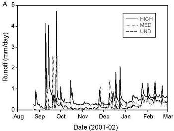 Figure 33. Stream runoff during a dry period (Aug 2001-Feb 2002) at three study catchments: UND = undeveloped, MED = medium density residential (1.6 houses ha-1, 6% impervious), HIGH = high density residential (2.8 houses ha-1, 11% impervious).
 From Burns D et al. 2005. Effects of suburban development on runoff generation in the Croton River basin, New York, USA. Journal of Hydrology 311:266-281. Reprinted with permission from Elsevier.
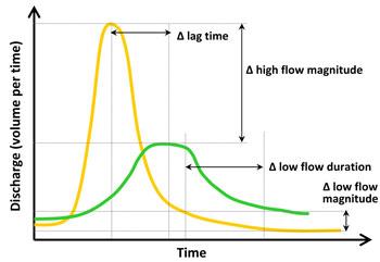 Figure 34. Hypothetical hydrographs for an urban stream (yellow) and a rural stream (green) after a storm, illustrating some common changes in stormflow and baseflow that occur with urban development. Other changes are listed at left.
These hydrologic changes can reduce habitat quality in urban streams and adversely affect stream biota. For example, high flows can scour organisms and substrate from streambeds, while low flows can reduce habitat area and volume. See the Flow Alteration and Physical Habitat modules for further details on biotic responses to these changes.
Baseflow in Urban Streams
Urbanization generally results in increased magnitude and frequency of peak flows. However, baseflow effects typically are more variable, with studies showing a range of responses in urban streams [Lerner 2002, Brandes et al. 2005, Meyer 2005, Roy et al. 2005 (Figure 35), Poff et al. 2006].
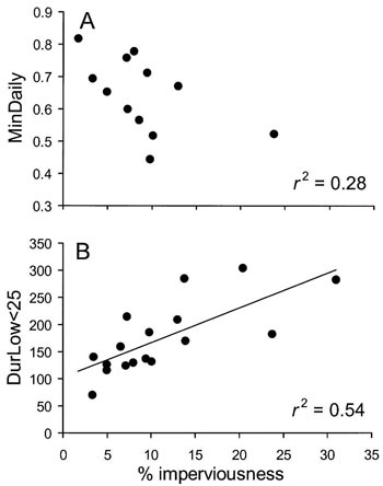 Figure 35. Linear regression models for baseflow variables showing highest correlations with subcatchment imperviousness: (A) minimum daily stage/mean daily stage during late spring; (B) maximum duration of low stage < 25th percentile during autumn. Of the nine baseflow variables tested across five seasons, only these two variables showed relationships with r2 > 0.25, and only in (B) was this relationship significant.
From Roy AH et al. 2005. Investigating hydrologic alteration as a mechanism of fish assemblage shifts in urbanizing streams. Journal of the North American Benthological Society 24(3):656-678. Reprinted with permission.
Decreases in baseflow may result from:
- Decreased infiltration due to increased impervious surfaces
- Increased water withdrawals (surface or ground)
These decreases may be offset, however, by increases in baseflow resulting from:
- Increased imported water supplies (i.e., interbasin transfers)
- Increased leakage from sewers and septic systems
- Increased leakage from water supply infrastructure
- Increased irrigation (e.g., lawn watering)
- Increased discharge of wastewater effluents
- Increased infiltration due to water collection in recharge areas
- Decreased evapotranspiration due to decreased vegetative cover
 Urban-related increases in baseflow can be especially evident in effluent-dominated systems, or streams and rivers in which wastewater effluents comprise a significant portion of baseflow volumes. For example:
- Discharge from two wastewater treatment plants accounted for at least 70% of river flow in the Bush River, SC in Summer 2002 (Andersen et al. 2004).
- Average effluent flow in the South Platte River, CO is 41% total streamflow; during low flow conditions, this can increase to 90% (Woodling et al. 2006).
As a result, changes in baseflow in these streams likely affect water and and sediment quality.
Water Withdrawals and Transfers
- Where the water comes from
- Surface water vs. groundwater
- Within catchment vs. imported from another catchment (i.e., water transfers)
- Direct intake from channel vs. from water supply reservoir
- Small vs. large streams
- Where the water goes
- Within catchment vs. exported to another catchment (i.e., water transfers)
- Small vs. large streams
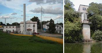 A New Orleans pump station that withdraws water from the Mississippi River and transfers it to a nearby treatment facility (left), and an intake structure for a water supply plant on the Duck River, TN (right).
Photo courtesy of Charlie Brenner (left) and USGS (right)
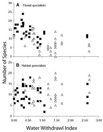 Figure 36. Richness estimates for (A) fluvial specialist and (B) habitat generalist fishes vs. water withdrawal index values [ln(permitted monthly average withdrawal/7Q10)]. Squares indicate sites where water intake was directly from channel; triangles indicate sites directly downstream from water supply reservoirs. Data were collected in 28 Georgia streams used for municipal water supplies, 2001-2003.
From Freeman MC & Marcinek PA. 2006. Fish assemblage responses to water withdrawals and water supply reservoirs in Piedmont streams. Environmental Management 38(3):435-450. Reprinted with permission from Springer. Freeman and Marcinek (2006) examined how surface water withdrawals for municipal water supplies affected stream fish assemblages in the Georgia Piedmont, using a withdrawal index that represented the amount of water withdrawn on a monthly average basis, relative to the 7-day, 10-year recurrence low flow in those streams (7Q10). They found that:
- Richness of fluvial specialist fishes (e.g., many minnows and darters) decreased as the amount of water withdrawn increased (Figure 36).
- This decrease generally occurred when permitted withdrawal rates exceeded approximately 0.5-1 7Q10-equivalent of water (Figure 36).
- As water withdrawals increased, so did the probability that sites would be classified as impaired based on their Index of Biotic Integrity scores.
- The type of water intake also was important, as reservoir presence (along with withdrawal rate and drainage area) were significant predictors of fluvial specialist richness.
Biotic Responses to Urban Flows
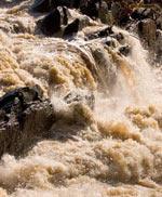 Photo courtesy of U.S. EPA Hydrologic changes associated with urbanization can directly and indirectly affect stream biota in many ways. Effects may include:
- Direct scour and dislodgement from benthic surfaces due to increased peak flows
- Altered physical habitat
- Changes in in-stream hydraulic conditions (e.g., water velocity, wetted channel area and duration)
- Changes in channel geomorphology
- Life cycle disruption due to changes in timing of flows
- Other flow-associated alterations (e.g., increased sediment, nutrient and contaminant delivery, changes in food resources)
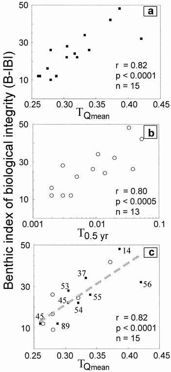 Figure 37. Relationship between benthic index of biological integrity for invertebrates and hydrologic variables TQmean (a, c) and T0.5 yr (b). In (c), numbers indicate % urban land cover (sites plotted as circles lacked land cover data). Note that lower values for TQmean and T0.5 yr indicate higher flow variablity and flashiness.
From Booth DB et al. 2004. Reviving urban streams: land use, hydrology, biology, and human behavior. Journal of the American Water Resources Association 40(5):1351-1364. Reprinted with permission.For example, Booth et al. (2004) examined how benthic index of biological integrity (B-IBI) scores were related to two flow metrics associated with urbanization:
- TQmean = the fraction of a year that mean daily discharge exceeds annual mean discharge
- T0.5 yr = the fraction of a multi-year period that a channel is exposed to flows greater than the 0.5-year flood
For both TQmean and T0.5 yr, low values indicate the prevalence high discharge peaks that both rise and dissipate sharply—that is, increased flashiness and flow variability.
Booth et al. (2004) found that:
- TQmean and T0.5 yr decreased as % total impervious area increased, indicating that urban streams experienced flashier hydrographs.
- B-IBI scores increased as TQmean and T0.5 yr increased, indicating that macroinvertebrate biotic condition was reduced in flashier streams (Figure 37a,b).
- Sites with ≥ 54% urban land cover fall below the main trendline, indicating that macroinvertebrate biotic condition was poorer than predicted by hydrologic conditions alone (Figure 37c).