Urbanization - Overview
What is Urbanization?
Urbanization refers to the concentration of human populations into discrete areas. This concentration leads to the transformation of land for residential, commercial, industrial and transportation purposes. It can include densely populated centers, as well as their adjacent periurban or suburban fringes (see Figure 1).
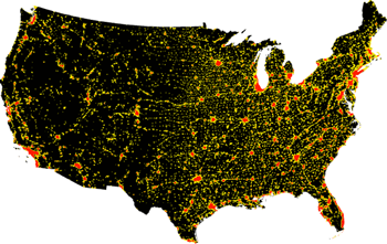 Figure 1. Urbanization map of the U.S. derived from city lights data (2009 data). Urban areas are colored red (represented of larger cities), while peri-urban areas are colored yellow. Image created by Flashback Imaging Corporation, under contract with NOAA and NASA [accessed 7/16/09].
- Core areas with population density ≥ 1,000 people per square mile, plus surrounding areas with population density ≥ 500 people per square mile (U.S. Census Bureau, for 2000 Census).
- Areas characterized by ≥ 30% constructed materials, such as asphalt, concrete and buildings (USGS National Land Cover Dataset).
| Measure | Description |
|---|---|
| % Total urban area | Area in all urban land uses |
| % High intensity urban | Area above some higher development threshold |
| % Low intensity urban | Area above some lower development threshold |
| % Residential | Area in residential-related uses |
| % Commercial/industrial | Area in commercial- or industrial-related uses |
| % Transportation | Area in transportation-related uses |
| % Total impervious area | Area of impervious surfaces such as roads, parking lots and roofs; also called impervious surface cover |
| % Effective impervious area | Impervious area directly connected to streams via pipes; also called % drainage connection |
| Road density | Road length per area |
| Road crossing density | # Road-stream crossings per area |
| Population density | # People per area |
| Household density | # Houses per area |
| Urban intensity indices | Multimetric indices combining a suite of development-related measures into one index value [e.g., the USGS national urban intensity index (NUII), based on housing density, % developed land in basin and road density] |
Why Does It Matter?
- Urban development has increased dramatically in recent decades, and this increase is projected to continue. For example, in the U.S. developed land is projected to increase from 5.2% to 9.2% of the total land base in the next 25 years (Alig et al. 2004).
- On a national scale, urbanization affects relatively little land cover, but it has a significant ecological footprint. Even small amounts of urban development can have large effects on stream ecosystems.
Key Pathways By Which Urbanization Alters Streams
- Riparian/channel alteration – Removal of riparian vegetation reduces stream cover and organic matter inputs. Direct modification of channel alters hydrology and physical habitat.
- Wastewater inputs – Human, industrial and other wastewaters enter streams via point (e.g., wastewater treatment plant effluents) and non-point (e.g., leaky infrastructure) discharges.
- Impervious surfaces – Impervious cover increases surface runoff, resulting in increased delivery of stormwater and associated contaminants into streams.
The Urban Stream Syndrome
Common effects of urbanization on stream ecosystems have been referred to as the "urban stream syndrome" (Walsh et al. 2005a).
Table 2 lists symptoms typically associated with the urban stream syndrome.
| Stressor Category | Symptom |
|---|---|
| Water/sediment quality | Increased nutrients |
| Increased toxics | |
| Altered suspended sediment | |
| Temperature | Increased temperature |
| Hydrology | Increased overland flow frequency |
| Increased erosive flow frequency | |
| Increased stormflow magnitude | |
| Increased flashiness | |
| Decreased lag time to peak flow | |
| Altered baseflow magnitude | |
| Physical habitat | Increased direct channel modification (e.g., channel hardening) |
| Increased channel width (in non-hardened channels) | |
| Altered pool depth | |
| Increased scour | |
| Decreased channel complexity | |
| Altered bedded sediment | |
| Energy sources | Decreased organic matter retention |
| Altered organic matter inputs & standing stocks | |
| Altered algal biomass | |
| Modified from Walsh CJ et al. 2005. The urban stream syndrome: current knowledge and the search for a cure. Journal of the North American Benthological Society 24(3):706-723. | |
 As the urban stream syndrome illustrates, these streams are simultaneously affected by multiple sources, resulting in multiple, co-occurring and interacting stressors. Thus, identifying specific causes of biological impairment in urban streams, or the specific stressors that should be managed to improve condition, is difficult. Some communities are approaching this challenge by managing overall urbanization, rather than the specific stressors associated with it—for example, by establishing total maximum daily loads (TMDLs) for impervious surfaces, rather than individual pollutants.
- Location and distribution of development
- Catchment vs. riparian
- Upstream vs. downstream
- Sprawling vs. compact
- Density of development
- Type of development and infrastructure
- Residential vs. commercial/transportation
- Stormwater systems
- Wastewater treatment systems
- Age of development and infrastructure
Urbanization and Biotic Integrity
Numerous studies have examined relationships between land use variables and stream biota. These studies have shown that urban-related land uses can significantly alter stream assemblages.
Land use variables considered include % urban land (in the catchment and in riparian areas), % impervious surface area (total and effective), road density and other measures of urbanization.
Biotic responses associated with these land use variables include (but are not limited to):
ALGAE
- Increased abundance or biomass
[Roy et al. 2003, Taylor et al. 2004, Busse et al. 2006] - Other changes in assemblage structure (e.g., diatom composition)
[Winter and Duthie 2000, Sonneman et al. 2001, Newall and Walsh 2005]
BENTHIC MACROINVERTEBRATES
- Decreased total abundance, richness or diversity
[Morley and Karr 2002, Moore and Palmer 2005, Walsh et al. 2007] - Decreased EPT (Ephemeroptera, Plecoptera, Trichoptera)
[Morley and Karr 2002, Roy et al. 2003, Riley et al. 2005, Walsh 2006] ![Plot of a measure of biotic homogenization [relative abundance of Appalachian highland endemic fishes – relative abundance of cosmopolitan fishes] on the first axis of a principal components analysis of three catchment land use variables](/sites/static/files/styles/large/public/2015-12/urban-biotic.jpg "Plot of a measure of biotic homogenization [relative abundance of Appalachian highland endemic fishes – relative abundance of cosmopolitan fishes] on the first axis of a principal components analysis of three catchment land use variables") Figure 2. Plot of a measure of biotic homogenization [relative abundance of Appalachian highland endemic fishes – relative abundance of cosmopolitan fishes] on the first axis of a principal components analysis of three catchment land use variables [1993 forest cover, forest cover change from 1970s–1990s, and urbanization intensity (normalized catchment building + road density)]. Sites with higher forest cover and lower urban intensity had more endemic taxa (e.g., fishes such as the Tennessee shiner and the mottled sculpin, above left), while sites with lower forest cover and higher urban intensity had more broadly distributed, generalist taxa (e.g., fishes such as the redbreast sunfish and central stoneroller, above right).
Figure 2. Plot of a measure of biotic homogenization [relative abundance of Appalachian highland endemic fishes – relative abundance of cosmopolitan fishes] on the first axis of a principal components analysis of three catchment land use variables [1993 forest cover, forest cover change from 1970s–1990s, and urbanization intensity (normalized catchment building + road density)]. Sites with higher forest cover and lower urban intensity had more endemic taxa (e.g., fishes such as the Tennessee shiner and the mottled sculpin, above left), while sites with lower forest cover and higher urban intensity had more broadly distributed, generalist taxa (e.g., fishes such as the redbreast sunfish and central stoneroller, above right).
From Scott MC. 2006. Winners and losers among stream fishes in relation to land use legacies and urban development in the southeastern US. Biological Conservation 127:301-309. Reprinted with permission from Elsevier.
Photos courtesy of Noel Burkhead, USGSIncreased abundance of tolerant taxa
[Jones and Clark 1987, Walsh et al. 2007]- Other changes in assemblage structure (e.g., functional fedding groups)
[Stepenuck et al. 2002, Smith and Lamp 2008] - Decreased quality of biotic index scores
[Kennen 1999, Morley and Karr 2002, DeGasperi et al. 2009]
FISHES
- Decreased abundance, biomass, richness or diversity
[Wang et al. 2003a, Bilby and Mollot 2008, Stranko et al. 2008] - Other changes in assemblage structure (e.g., reproductive guilds)
[Stepenuck et al. 2002, Roy et al. 2007, Helms et al. 2009] - Decreased quality of biotic index scores
[Snyder et al. 2003, Miltner et al. 2004, Morgan and Cushman 2005] - Increased biotic homogenization (replacement of more endemic, specialist fishes with more broadly distributed, generalist fishes)
[Scott 2006 (Figure 2), Walters et al. 2009]
Catchment vs. Riparian Urbanization
- Catchment: the entire catchment area above the site
- Riparian: the entire riparian area in the catchment above the site
- Reach: the riparian area for a relatively short distance above the site
 Figure 3. Scatterplots of the threshold effect of developed land on macroinvertebrate assemblage composition (Bray-Curtis dissimilarity expressed as nonmetric multidimensional scale [nMDS] Axis 1 scores), for (A) % developed land in watershed, (B) % developed land within 250-m radius buffer of site, (C) % developed land in watershed weighted by its inverse distance (IDW) to site. Dotted lines indicate the cumulative probability of an ecological response to increasing % developed land. Sites within the watershed-scale threshold zone of 21-32% developed land in (A) are highlighted in black in all panels.
 From King RS et al. 2005. Spatial considerations for linking watershed land cover to ecological indicators in streams. Ecological Applications 15(1):137-153. Reprinted with permission.
- For % developed land in the watershed (Figure 3A), there was an apparent threshold between 21-32% where the probability of assemblage alterations increased rapidly. Once >32% of the watershed was developed, all macroinvertebrate assemblages were affected.
- When % developed land in the 250-m buffer was considered (Figure 3B), this threshold shifted left and all macroinvertebrate assemblages were affected once >22% of land in the 250-m buffer was developed.
- A similar pattern was seen when developed land in the watershed was inverse-distance weighted (i.e., development closer to the focal site was weighted more than development farther away; Figure 3C). Then, the threshold for macroinvertebrate effects occurred between 18-23%.
The relative importance of development at different scales varies across studies (e.g., Sponseller et al. 2001, Wang et al. 2001, Morley and Karr 2002, Roy et al. 2003, Snyder et al. 2003, Schiff and Benoit 2007). It likely depends, at least in part, on the stressors considered (Allan 2004).
For example, some stressors associated with urbanization (e.g., changes in flow) are highly dependent on catchment-scale processes, while other stressors (e.g., changes in basal energy sources) are more affected by reach-scale processes.