Analytical Examples
This section presents five (5) examples illustrating the use of data analysis to support different types of evidence. Each example provides details about the analysis technique used and the type of evidence supported. These include:
- Spatial Co-occurrence with Regional Reference Sites (Example 1).
- Verified Prediction: Predicting Environmental Conditions from Biological Observations (Example 2).
- Stressor-Response Relationships from Field Observations (Example 3).
- Stressor-Response Relationships from Laboratory Studies (Example 4).
- Verified Prediction with Traits (Example 5).
Example 1. Spatial Co-occurrence with Regional Reference Sites
On this Page
Introduction
We would like to determine whether stream temperatures observed at an Oregon test site are higher than those at regional reference sites. If temperatures at the test site are higher than reference expectations, then we can conclude that increased temperature spatially co-occurs with the observed impairment. Conversely, temperatures at the test site that are comparable to temperatures at regional reference sites would suggest that increased temperature does not spatially co-occur with the observed impairment.
Data
The Oregon Department of Environment Quality (ORDEQ) deployed continuous temperature monitors in streams from 1997-2002. These temperature monitors recorded hourly temperature measurement which were then summarized as seven day average maximum temperatures in degrees C (7DAMT). Sites were also characterized by the geographic location (latitude and longitude), elevation, and catchment area. Reference sites were designated in Oregon based on land use characteristics.
Analysis and Results
Scatter plots are first used to examine the variation of stream temperature with different natural factors. The factors that are chosen (e.g., elevation, geographic location) must not be associated with local human activities. This initial data exploration suggests that stream temperature in reference sites are inversely related with both elevation and latitude (Figure 1). Next, regression analysis is used to model stream temperature as a function of elevation and latitude.
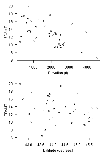 Figure 1. Scatter plots comparing 7 day average maximum temperature (7DAMT) with elevation (top plot) and latitude (bottom plot). We would like to determine whether stream temperatures observed at a test site in Oregon are higher than those observed at comparable regional reference sites. If temperatures at the test site are higher than reference expectations, then we can conclude that increased temperature spatially co-occurs with the observed impairment. Conversely, temperatures at the test site that are comparable to temperatures at regional reference sites would suggest that increased temperature does not spatially co-occur with the observed impairment.
Both elevation and latitude are statistically significant (p < 0.05) predictors of stream temperature. The model explains approximately half of the overall variability in stream temperature. This model can be used to predict the reference expectations for stream temperature at other sites. That is, the reference expectation for temperature can be calculated as follows:
t = 76.6 - 0.0019E - 1.36L
where t is the stream temperature, E is the elevation of the site in feet, and L is the latitude of the site in decimal degrees.
Now, suppose a biologically impaired test site of interest is located at a latitude of 43 degrees N and an elevation of 1000 ft. We monitored stream temperature at this site and found that the seven day average maximum temperature at the site was 22 °C. Temperature is listed as a candidate cause of impairment at this site, and so we would like to know whether stream temperature at the site is elevated relative to the regional reference conditions. The reference expectation for stream temperature can be predicted as follows,
t = 76.6 - 0.0019(1000) - 1.36(43)
which gives a predicted reference temperature of 16.4 degrees. Most statistical software will also provide prediction intervals at a specified probability. For this case, 95% prediction intervals around the mean value are 11.4 and 21.4 degrees. Hence, the observed temperature is greater than temperatures we would expect for 95% of reference samples collected at the same elevation and latitude, suggesting that stream temperature is indeed elevated at the test site. We would conclude that at this test site, elevated stream temperature co-occurs with the biological impairment.
The CADStat Regression Prediction tool performs all of these calculations, and also determines whether conditions at test sites are within the range of experience of the set of reference sites.
How Do I Score This Evidence?
Elevated temperatures co-occurs with the biological impairment so we would score this evidence as +.
Example 2. Verified Prediction: Predicting Environmental Conditions from Biological Observations
On this Page
Introduction
We would like to determine whether observed changes in the macroinvertebrate assemblage composition at a test site in Oregon is consistent with a hypothesis that temperature has increased at the site. That is, if increased temperature is a stressor at the test site, we predict that the temperature inferred from the impaired macroinvertebrate assemblage is higher than expected. For this example, we establish our expectations for the inferred temperature using a set of regional reference sites.
Data
Macroinvertebrate samples and temperature measurements were collected from small streams across the western United States by the U.S. EPA Environmental Monitoring and Assessment Program.
The Oregon Department of Environment Quality (ORDEQ) deployed continuous temperature monitors in streams from 1997-2002. These temperature monitors recorded hourly temperature measurements that were summarized as seven-day average maximum temperatures (7DAMT). Macroinvertebrate samples were also collected from these sites. Sites were characterized by the geographic location (latitude and longitude), elevation, and catchment area. Reference sites were designated in Oregon based on land use characteristics.
Analysis and Results
Inference Model Development and Validation
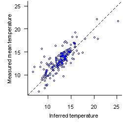
Figure 2. Temperature inferred from macroinvertebrate data versus measured mean temperature (7 day average maximum temperature). Dashed line shows a 1:1 correspondence.Relationships between the probability of capture of different macroinvertebrate taxa and stream temperature were estimated in the EMAP data set using logistic regression (Yuan 2007). These models were then combined with observations of different taxa in the Oregon data to predict stream temperature at each of the Oregon sites.
The accuracy with which the EMAP models predicted Oregon stream temperatures was assessed by plotting temperature inferred from the macroinvertebrate assemblage versus directly measured mean temperature (Figure 2). Agreement between inferred and directly measured temperatures was strong.
Controlling for Natural Variability
The factors that are chosen for the predictive model (e.g., elevation, geographic location) must not be associated with human activities. This initial data exploration suggested that stream temperature in reference sites varies with both elevation and latitude (Figure 3).
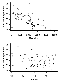 Figure 3. Relationships between inferred temperature and elevation (top) and latitude (bottom).A multiple linear regression model was used to quantify the relationship between inferred temperature and latitude and elevation at reference sites. Both elevation and latitude are statistically significant (p < 0.05) predictors of stream temperature, and the model explains approximately half of the overall variability in inferred stream temperature. This model can be used to predict the reference expectations for inferred stream temperature at other sites. That is, the reference expectation for inferred temperature can be calculated as follows:
where ti is the stream temperature, E is the elevation of the site in feet, and L is the latitude of the site in decimal degrees.
Site Assessment
Since the inference model seemed to provide accurate predictions of stream temperature, inferred temperature can be used to inform the verified prediction type of evidence. That is, we hypothesize that if temperature is the cause of impairment then temperatures inferred from the impaired macroinvertebrate assemblage will be higher than expected.
At the biologically impaired test site of interest we collected a macroinvertebrate sample and used the EMAP inference models to infer temperature at the test site as 21°C based on the macroinvertebrate assemblage. The biologically impaired site is located at an elevation of 1000 feet and latitude of 43° North. The expected inferred stream temperature at the site is predicted using the regression relationship developed from regional reference conditions,
ti = 50.3 - 0.0013 (1000) - 0.82( 43)
which gives a predicted reference inferred temperature of 13.7°C. 95% prediction intervals around this mean value are 10.5°C and 17.2°C, so the EMAP inferred temperature of 21°C, based on the collected macroinvertebrate assemblage, is well outside the predicted range of 95% of inferred temperatures at similar reference sites. This finding suggests that inferred stream temperature is indeed elevated at the test site. Hence, the macroinvertebrate assemblage at the test site is one that is characteristic of much warmer streams than we would expect for a stream at this elevation and latitude. At this test site, we have verified our prediction that the observed macroinvertebrate assemblage is consistent with temperatures being higher than expected.
The CADStat PECBO and Regression Prediction tools perform all the calculations described in this example.
How Do I Score This Evidence?
Predictions of increased biologically-inferred temperatures have been verified (+).
References
- Yuan LL (2007) Maximum likelihood method for predicting environmental conditions from assemblage composition: The R package bio.infer. Journal of Statistical Software 22: Article 3.
Example 3. Stressor-Response Relationships from Field Observations
On this Page
Introduction
We would like to determine whether water quality variables in Long Creek, Maine (U.S. EPA 2007) are associated with three observed changes in the aquatic invertebrate community relative to the reference stream: a decrease in Ephemeroptera, Plecoptera and Trichoptera (EPT) richness; an increase in percent non-insect taxa; and a shift towards increased pollution tolerance, estimated using Hilsenhoff's Biotic Index (HBI) (Hilsenhoff 1987, 1988).
In this example, we present analyses relevant to two candidate causes, ionic strength (measured using specific conductivity), and zinc. If specific conductivity (or zinc) is not associated with the biological responses in the expected direction, this evidence would weaken the argument for ionic strength (or zinc) being a cause of the observed biological changes. Conversely, if specific conductivity (or zinc) is associated with the biological responses in the expected direction, this evidence would somewhat support the argument that ionic strength (or zinc) is the cause of the observed changes.
These associations can provide only weak support for a causal argument because other stressors may be correlated with increased conductivity (or zinc), and are not controlled for in this analysis. For this reason, it is important to conduct this analysis for as many of the candidate causes as possible.
Data
Biological and water chemistry data from 8 sites along Long Creek and a similar but unimpaired reference stream, are used in this example.
Biological metrics were calculated from macroinvertebrate rockbag samples deployed throughout the study area beginning August 5-6, 1999, for a period of 32 days, following standard Maine Department of Environmental Protection (MEDEP) protocol (Davies and Tsomides 2002).
Water chemistry measurements of conductivity and zinc were made from baseflow water samples collected by MEDEP on three days in August 2000. Methods and analyses are described in MEDEP (2002). Here, the analysts assume that the differences in the collection dates for biological samples (1999) and for water chemistry samples (2000) did not affect observed relationships. Ideally, additional data would be collected as a follow-up to validate this assumption.
Analysis and Results
The data were analyzed using scatter plots (Figure 4). The project team interpreted the scatter plots by looking for linear and curvilinear trends in the data. Because only one data point from each site was available, the plots were not used to make judgments about individual sites or stream reaches. Instead, the plots were used to characterize trends across the two watersheds.
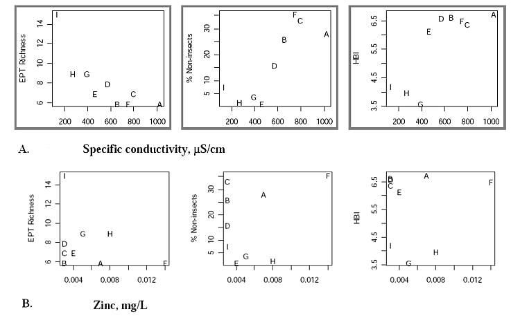 Figure 4. Scatter plots showing the association between EPT richness, percent benthic non-insects and HBI and specific conductivity (upper plot, A) and zinc (lower plot, B). Plots judged to exhibit a linear or non-linear association are outlined in gray.
Sample sites and methods are described in the case study report Long Creek (USEPA 2007).
The visual interpretation of the scatterplots was supplemented with correlation coefficients (Table 1). Correlation coefficients were not evaluated for significance because of the small sample size and pseudo-replication of sites. Rather, consistent correlations of relatively large magnitude for all three biological responses were considered by the analysts to provide some support for ionic strength as a candidate cause. When evaluating this evidence, it is worth noting again that both analyses hinge on the assumption that samples of water chemistry taken in August 2000 are similar to exposures experienced by organisms in August 1999.
| Specific conductivity | Zinc | |
|---|---|---|
| EPT Richness | -0.86 | -0.21 |
| % non-insects | 0.78 | 0.026 |
| HBI | 0.78 | -0.15 |
How Do I Score This Evidence?
Associations between specific conductivity and all three biological responses were apparent and in the expected direction. We would score this evidence as + for each of the biological responses.
There were no clear associations between zinc and any of the three biological responses. We would score this evidence as - for each of the biological responses.
References
- Davies SP, Tsomides L (2002) Methods for biological sampling and analysis of Maine's rivers and streams. Maine Department of Environmental Protection, Augusta ME. DEP LW0387-B2002.
- Hilsenhoff WL (1987) An improved biotic index of organic stream pollution. Great Lakes Entomologist 20:31-39.
- Hilsenhoff WL (1988) Rapid field assessment of organic pollution with a family level biotic index. Journal of the North American Benthological Society 7(1):65-68.
- MEDEP (2002) A biological, physical, and chemical assessment of two urban streams in southern Maine: Long Creek and Red Brook. Maine Department of Environmental Protection, Augusta ME. DEP-LW0572.
- U.S. EPA (2007) Causal Analysis of Biological Impairment in Long Creek: A Sandy-Bottomed Stream in Coastal Southern Maine. U.S. Environmental Protection Agency, Office of Research and Development, National Center for Environmental Assessment, Washington DC. EPA-600-R-06-065F.
Example 4. Stress or-Response Relationships from Laboratory Studies
On this Page
Introduction
In this example, we ask whether organisms in Long Creek, Maine (U.S. EPA 2007) are exposed to a candidate cause (zinc) at quantities or frequencies sufficient to induce observed biological effects. We use results from laboratory studies to evaluate whether zinc in the water column under base flow conditions reached concentrations that could explain the observed decrease in Ephemeroptera, Plecoptera and Trichoptera (EPT) richness. The comparison of laboratory and field data can be performed in two ways.
- Most commonly, effective concentrations from laboratory data are compared to ambient concentrations at the affected site. If zinc concentrations associated with similar types of effects in the laboratory are similar to or lower than concentrations that have been shown to occur at the affected site, this would provide evidence that zinc concentrations are high enough to cause the effects.
Conversely, if zinc concentrations associated with similar types of effects in the laboratory are much higher than those at the affected site, then the case for zinc would be weakened. Either some other stressor is the cause of the observed decline, or zinc is acting jointly with another cause to produce the effect.
- We can also compare the magnitude of effects observed at the site with the magnitude of effects observed in the laboratory at concentrations equal to ambient concentrations. If the magnitude of effects at the site are much greater than would be predicted from the laboratory concentration-response relationship, then we would conclude that either zinc concentrations are not high enough to have caused the effects, or the laboratory organisms or endpoints are not as sensitive as the organisms or responses at the affected site. If magnitude of effects observed at the site is approximately equal to those predicted from the laboratory concentration-response relationship, then this would support the argument that zinc is the cause of the effects. Finally, if the magnitude of effects observed at the site is much less than predicted from laboratory studies, we would conclude that some physical factor (e.g., dissolved organic matter) or some biological process (e.g., replacement of sensitive insect species by tolerant species) may be reducing the effect in the field.
Data
This example uses summaries of laboratory toxicity test results and compares these summaries with data from the site.
Laboratory Toxicity Data
Two approaches were used to summarize laboratory results. First, U.S. EPA's chronic criterion value for zinc was used to represent sublethal effects and effects of extended exposures. The chronic criterion value for zinc at 100 mg/L hardness (as CaCO3) is 0.12 mg/L. A chronic value for an EPT insect would be preferable, but none were available.
It was necessary to generate SSDs with data for total metals because greater than 90% of freshwater metals data in ECOTOX are reported as total metals. Free ion or dissolved metal concentrations would be more appropriate indicators of actual toxic exposure and be more relevant to the dissolved metal concentrations reported for Long Creek. However, this is a relatively minor problem, because nearly all metals in laboratory tests are dissolved.
SSDs were generated using LC50 data. Since an LC50 is a concentration that kills half of the organisms in a test population, one would expect to observe a reduction in the abundance of some species when water concentrations equal the LC50 for that species. Data used in generating SSDs do not represent specific species present at the study area. Toxicity data are generally not available for site-specific taxa due to the diversity of species occurring in the wild and the need to perform toxicity tests with well characterized organisms.
Site Data
Biological and water chemistry data from two sites along Long Creek are used in this example. EPT richness was calculated from macroinvertebrate rockbag samples deployed throughout the study area beginning August 5-6 1999, following standard Maine Department of Environmental Protection (MEDEP) protocol (Davies and Tsomides 2002).
Baseflow water samples were collected by MEDEP on three days in August 2000. Methods and analyses are described in MEDEP (2002).
Analysis and Results
The laboratory results were compared to site data by graphically comparing the proportion of decrease in EPT richness, relative to the reference site, and impaired site zinc concentrations. In addition, the SSD was used to identify 0.087 as a benchmark concentration of 10% at which 10% of species would be expected to experience lethal effects.
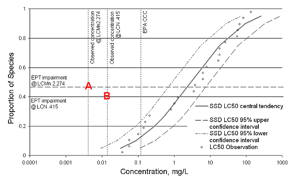 Figure 1. Comparison of site observations from Long Creek with the EPA criterion continuous concentration for Zn (EPA CCC) and a species sensitivity distribution. Points A and B mark corresponding biological observations and Zn concentrations from Sites LCMn2.274 and LCN .415, respectively.
Discussion
- The organisms and endpoints measured in the laboratory are relevant to EPT richness.
- The laboratory exposures are relevant to the exposures encountered by organisms in the field.
- Measured baseflow concentrations of zinc in August 2000 were similar to unmeasured concentrations in August 1999.
How do I score this evidence?
Measured concentrations are all below the EPA criterion continuous concentration. The measured concentrations at the site fall below the 10% benchmark derived from the SSD. Points corresponding to the observed impairment occur at concentrations below the lower confidence limits on the SSD curve. This weakens the case that zinc caused the observed decreases in EPT, giving a score of - (one minus).
References
- Davies SP, Tsomides L (2002) Methods for biological sampling and analysis of Maine's rivers and streams. Maine Department of Environmental Protection, Augusta ME. DEP LW0387-B2002.
- MEDEP (2002) A biological, physical, and chemical assessment of two urban streams in southern Maine: Long Creek and Red Brook. Maine Department of Environmental Protection, Augusta ME. DEP-LW0572.
- U.S. EPA (2007) Causal Analysis of Biological Impairment in Long Creek: A Sandy-Bottomed Stream in Coastal Southern Maine. U.S. Environmental Protection Agency, Office of Research and Development, National Center for Environmental Assessment, Washington DC. EPA-600-R-06-065F.
Example 5. Verified Prediction with Traits
On this Page
Introduction
In causal analysis we find that trait information is well suited to a type of evidence called verified prediction, where the knowledge of a cause's mode of action permits prediction and subsequent confirmation of previously unobserved effects. In this application, we would predict changes in the occurrence of different traits we would expect to occur if a particular stressor was present and causing biological effects. If we found that these traits do indeed occur at the impaired site, our prediction is verified and the causal hypothesis is supported by that evidence.
Analysis and Results
Analytical approaches range from basic comparisons of measurements to more formal statistical tests (see page on establishing differences from expectations). Incorporating predictions of traits into causal analysis is an area of active research, and so we present a hypothetical example below.
Existing information about the relationship between a trait and environmental gradients can be used to predict how the occurrence of a trait will differ between the test site and reference expectations. The occurrence of a trait in a community from test site is compared with a community from a reference site. If the predicted occurance of a is supported, the result would support a claim of verified prediction.
We illustrate this with an example of clinger relative richness and sediment in streams across the eastern United States. Existing literature indicates that the relative richness of clingers decreases with increased bedded sediment (Figure 5, Pollard and Yuan 2010). 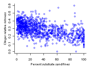 Figure 5. Relative richness of clingers versus percent substrate sand/fines. Data from streams of the western United States.Based on this existing relationship, we predict that if bedded sediments are a cause of impairment in a test stream, then the relative richness of clingers should be lower in the test stream than in comparable reference streams. Then, we compare the trait data from our reference site to the trait data from the test site. If the test site has fewer clingers than the reference site, the general prediction is confirmed.
How Do I Score This Evidence?
If the predicted pattern is observed (here, if the test site had fewer clingers than the reference site), the type of evidence "verified prediction" is scored as supported (+). If multiple predictions were verified or if the predictions were highly specific, the evidence may be convincing (+++).
References
- Abell R, Thieme ML, Revenga C, Bryer M, Kottelat M, Bogutskaya N, Coad B, Mandrak N, Balderas SC, Bussing W, Stiassny MLJ, Skelton P, Allen GR, Unmack P, Naseka A, Ng R, Sindorf N, Robertson J, Armijo E, Higgins JV, Heibel TJ, Wikramanayake E, Olson D, Lopez HL, Reis RE, Lundberg JG, Sabaj Perez MH, Petry P (2009) Freshwater ecoregions of the world: a new map of biogeographic units for freshwater biodiversity conservation. BioScience 58:403-414.
- Pollard AI, Yuan LL (2010) Assessing the consistency of response metrics of the invertebrate benthos: a comparison of trait- and identity-based measures. Freshwater Biology 55:1420-1429.