PECBO Appendix
Overview
Can the Biota at a Site Tell Us Environmental Conditions at that Site?
This module provides statistical tools for predicting environmental conditions from biological observations, or PECBO, and provides some of the ecological and statistical theory that underlie this method.
Different taxa require different environmental conditions to persist. From the figures shown below, we can see that the riffle beetle, Heterlimnius, is most frequently found in streams that are approximately 8° C (Figure 1), while the stonefly, Malenka, prefers warmer streams (~12° C) (Figure 2). If we knew the environmental preferences (i.e., the taxon-environment relationships) of many different taxa, we might be able to infer the environmental conditions at a site only from the biota that are observed at the site.
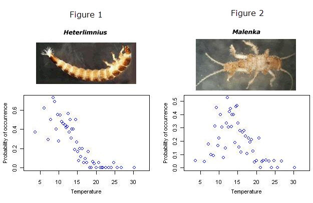 Probabilities of occurrence of Heterlimnius and Malenka along a temperature gradient. Each symbol represents the average frequency of occurrence within approximately 20 samples around the indicated temperature. Horizontal axis in units of °C.Inferring environmental conditions from biological observations can be very useful for stressor identification because they provide a biologically-based measure of environmental conditions at a site. Thus, these inferences can often provide another, alternate line of evidence that can strengthen a case made with other measurements.
The Helpful Links box provides additional introductory information including an overview of the Appendix's organization, and a discussion of the underlying theory and useful defintions.
Overview
This section provides a detailed step-by-step guide for inferring environmental conditions from your local benthic macroinvertebrate data. These inferences use pre-existing taxon-environment relationships for different environmental variables (e.g., stream temperature and bedded fine sediment) that are available in the CADDIS database.
It is assumed in this section that the user has some experience with the command line interface of R and is interested in thoroughly understanding the steps involved in predicting environmental conditions from biological observations.
- If you have no experience with R, you may want to use the tool for biological inferences provided in Menu-driven Package of Several Data Visualization and Statistical Methods (CADStat).
- A brief review of R command line syntax is provided in the R Command Line Tutorial.
- Download the library of R scripts and the appropriate taxon-environment dataset
- Standardize the taxonomy of your biological observations
- Assign operational taxonomic units (OTUs) to your biological observations
- Compute Biological Inferences for each of your sites
Overview
Taxon-environment relationships estimated from local data can potentially provide more accurate environmental inferences than the regional-scale relationships provided in the CADDIS database. In this section, different statistical methods for estimating taxon-environment relationships are presented. Additional details are on each topic can be found in the Helpful Links box on the right-hand side of this page. More extensive details on each of these methods can be found in Yuan (2006).
Before computing taxon-environment relationships, it is important to consider whether you have sufficient data by reviewing biological and environmental data requirements.
The simplest approaches for estimating taxon-environment relationships represent the entire relationship using a single value. This single value can quantify the average conditions that are preferred by a taxon (i.e., see Central Tendencies ), or it can quantify the limiting environment conditions under which a taxon can persist (see Environmental Limits).
Methods that estimate the entire taxon-environment relationship (rather than a single value) are somewhat more involved, requiring that one solve a regression equation that relates taxon occurrences or abundances to different values of one or more environmental variables. However, once taxon-environment relationships are estimated, one can usually develop more accurate biological inferences.
- Parametric Regressions
- Nonparametric Regressions
- How well does the model fit (see Assessing Model Fit)?
- Are there errors in the environmental variables (see Measurement Error)?
- Should survey design weights be incorporated into the regressions (see Survey Weighting)?
When entire taxon-environment relationships are available, they can be used to classify taxa into broad categories (e.g., tolerant or intolerant to elevated fine sediments); these classifications can be useful for building biological metrics. Placing taxa into tolerance categories provides guidance on classification of taxa tolerances.
Once taxon-environment relationships have been estimated, different inference methods can be applied to estimate environmental conditions at sites using biological observations.
References
- Yuan LL (2006) Estimation and application of macroinvertebrate tolerance values. U.S. Environmental Protection Agency, Office of Research and Development, Washington DC. EPA/600/P-04/116A.
Overview
In this section, we examine different statistical methods for inferring environmental conditions at the site if a biological sample is available and if taxon-environment relationships are available. Additional details on each method can be found from the Helpful Links box.
Weighted Average Inferences. If single value descriptors (e.g., weighted averages) have been used to characterize taxon-environment relationships, then the only approach that one can use to infer conditions at a new site is by computing the average value of the descriptors for taxa observed at a site. Weighted average inference estimates site conditions as the average of the descriptors of taxa observed at the site.
Maximum Likelihood Inferences. If entire taxon-environment relationships are available, maximum likelihood inference provides a more powerful and more accurate means of inferring the conditions at a site.
Categorical Tolerance Data. Finally, if taxa have been classified into tolerant and intolerant categories, traditional biological metrics can be used to characterize the site.
Overview
This section provides short scripts (i.e., programs) that perform the simpler statistical analyses described in this module. R, a free software package for statistical computations, is used for these examples. A link to a brief R Command Line Tutorial is provided in the Helpful Links box, as is the link to the home webpage for the R Project for Statistical Computing.
This section progresses sequentially through different scripts for computing and applying taxon-environment relationships. If you wish to run the scripts provided here, you should first visit the R Project for Statistical Computing web page and install R on your computer. Note: if you use S-Plus, many of these scripts also will work in S-Plus. However, some minor differences in command format between the two programs may cause unpredictable behavior.
All of the scripts can be downloaded as text files and directly "sourced" in R; the sample data used to demonstrate the scripts also are available by clicking the Download R Scripts and Sample Data from the Links Box.
Alternatively you can directly access individual scripts from the Quick Links box.
More complex scripts are provided in the R library bio.infer.